Chapter 44
Vacuum Structure as Constraint Field

The Casimir Effect
Author: Mark Higgins
© Mark Anthony Higgins 11 October 2025
Revised Date: 25 June 2026
Audio Overview

Introduction

The vacuum is often described in modern physics as empty space containing fluctuating quantum fields. Within quantum field theory, the vacuum is not truly empty but represents the lowest-energy state of all interacting fields. Virtual particles, vacuum fluctuations, and zero-point energy emerge from this picture and have successfully explained many observed phenomena.

Within the Holographic Space-Time (HST) framework, however, the vacuum is reinterpreted in a fundamentally different way.

Rather than viewing the vacuum as a sea of fluctuating particles or latent energy states, HST proposes that the vacuum is a constraint field: a geometric coherence structure that governs which boundary configurations are permitted and which are forbidden.

In this view, the vacuum is not something that contains physical objects. Instead, it is the underlying rule-set that determines how physical structures may form, evolve, propagate, and interact.

The vacuum therefore becomes an active participant in physical reality—not through forces or particles—but through the enforcement of coherence constraints across boundary geometries.

44.1 The Problem with Empty Space

Classical physics treated empty space as a passive background.

Objects moved through space.

Fields existed within space.

Space itself played little dynamic role.

Quantum theory altered this picture by introducing vacuum fluctuations, suggesting that even apparently empty regions possess activity.

Yet several conceptual questions remain:

Why do vacuum fluctuations possess specific structures?
Why are certain field configurations stable while others are not?
Why do particles exhibit preferred modes of existence?
Why do coherent structures emerge from apparently random fluctuations?

The standard framework describes the behaviour of the vacuum mathematically but does not fully explain why those constraints exist.

HST approaches the problem from a different direction.

Instead of asking:

What exists inside the vacuum?

HST asks:

What structures are permitted by the vacuum?

This inversion shifts the vacuum from an energy reservoir to a coherence regulator.

44.2 Vacuum as a Constraint Field

In HST every physical system exists upon evolving boundary structures.

These boundaries possess finite coherence capacity.

Not all configurations can exist simultaneously.

The vacuum therefore acts as the global constraint geometry governing allowable boundary states.

Formally:

\[ V_c = C \left( B_t \right) \]

Where:

  • VcV_c = vacuum constraint field
  • BtB_t = boundary geometry
  • C\mathcal{C} = coherence constraint operator

The vacuum field does not generate particles.

Instead it defines the admissible solution space.

Only configurations satisfying coherence constraints may persist.

Thus:

\[ S_{\mathrm{allowed}} = \left\{ S_i \;\middle|\; \Gamma \left( S_i \right) \geq \Gamma_{\mathrm{min}} \right\} \]

where:

  • SiS_i = candidate structures
  • Γ\Gamma = coherence measure
  • Γmin\Gamma_{min} = minimum stability threshold

Structures falling below the threshold are naturally suppressed.

44.3 Constraint Selection and Stability

Consider a vibrating membrane.

Many vibration patterns are mathematically possible.

Only specific standing-wave patterns remain stable.

The membrane itself acts as a constraint field.

The vacuum performs an analogous role for reality.

Every possible field configuration may be considered a candidate coherence pattern.

The vacuum continuously filters these possibilities.

Stable structures survive.

Unstable structures decay.

The process is not arbitrary.

It follows directly from geometric compatibility.

Thus:

\[ \mathrm{Stability} \propto \mathrm{Compatibility} \left( B_t, S_i \right) \]

The vacuum therefore behaves as a universal selection mechanism operating on boundary coherence.

Telephone:
01377 236594

44.4 Vacuum and Particle Existence

In standard quantum theory particles emerge as excitations of fields.

HST reframes this concept.

Particles emerge as stable coherence knots permitted by the vacuum constraint field.

A particle exists only when:

\[ \Gamma \left( S_i, V_c \right) \geq \Gamma_{\mathrm{min}} \]

where the vacuum provides the acceptance criteria.

This interpretation naturally explains why:

  • electrons possess fixed properties
  • photons propagate predictably
  • stable matter persists
  • unstable particles decay

The vacuum is continuously evaluating structural compatibility.

Existence becomes a consequence of constraint satisfaction.

44.5 Why the Vacuum Appears Empty

The vacuum appears empty because stable structures are absent.

Yet the constraint field remains present.

An analogy is useful.

A chessboard without pieces appears empty.

However:

  • movement rules still exist
  • legal positions still exist
  • constraints still operate

The board is not physically occupied, but its governing structure remains active.

Similarly:

  • the vacuum may contain no particles
  • the coherence rules remain present

Thus emptiness is not absence.

It is unoccupied constraint geometry.

44.6 Vacuum Energy Reinterpreted

Traditional physics attributes measurable effects such as:

  • the Casimir Effect
  • zero-point energy
  • vacuum polarization

to vacuum fluctuations.

HST offers an alternative interpretation.

These effects emerge from changes in constraint availability.

When boundaries are introduced:

\[ B_t \rightarrow B_t' \]

the set of allowable coherence modes changes:

\[ M_t \rightarrow M_t' \]

This modifies coherence density:

\[ \rho_C \rightarrow \rho_C' \]

Observable forces arise from the redistribution of permitted configurations rather than particle creation from nothing.

Thus vacuum energy becomes:

\[ E_V \propto \Delta C \]

where:

\[ \Delta C \]

represents the change in available coherence states.

44.7 Vacuum as the Foundation of Geometry

The deepest implication of HST is that geometry itself emerges from vacuum constraints.

Space is not a container.

Space is the visible projection of permissible coherence relationships.

The vacuum defines:

  • allowable curvature
  • allowable propagation
  • allowable information transfer
  • allowable structural formation

In this sense the vacuum is closer to a geometric operating system than an empty region.

Reality emerges from the execution of those constraints.

Telephone:
01377 236594

44.8 Constraint Fields and the Emergence of Physical Law

Physical laws appear universal because they are expressions of the same underlying vacuum constraint geometry.

Gravity becomes:

Constraint-DrivenCurvature


Electromagnetism becomes:

Constraint-DrivenFieldAlignment


Quantum phenomena become:

Constraint-DrivenStateSelection

The vacuum therefore unifies seemingly distinct phenomena under a common principle:

Physical behaviour emerges from coherence constraints acting upon evolving boundary structures.

44.9 HST Interpretation

Within Holographic Space-Time theory, the vacuum is not empty space and not a sea of fluctuating particles.

It is a global coherence constraint field that continuously governs which structures may exist.

Particles are permitted coherence knots.

Fields are permitted coherence gradients.

Forces are responses to constraint imbalances.

Geometry itself emerges from permissible boundary relationships.

The vacuum therefore becomes the deepest structural layer of physical reality—not a substance, not an object, and not a container, but the coherence framework from which all observable structures emerge.

In HST, reality exists because the vacuum continually separates the possible from the impossible.

FLOW VacuumStructure_AsConstraintField

VERSION 1.0

AUTHORS
    Mark Higgins
    Sky Recursive AI

PURPOSE
    Model the vacuum not as empty space, but as an active constraint field that
    determines which boundary configurations, coherence modes, particles, and
    field structures are permitted to persist.

DOMAIN
    HST Physics
    Vacuum Structure
    Boundary Coherence
    Constraint Fields

STATE_MODEL
    B_t              = Boundary geometry at time t
    V_C              = Vacuum constraint field
    C_t              = Coherence map
    M_t              = Candidate vacuum modes
    Γ(M_i, V_C)      = Compatibility of mode M_i with vacuum constraints
    Γ_min            = Minimum coherence threshold
    K_M(M_i)         = Structural cost of mode M_i
    C_V              = Vacuum coherence capacity
    M_allowed        = Modes permitted by vacuum constraints
    M_suppressed     = Modes rejected by vacuum constraints
    ρ_C              = Coherence density
    Δρ_C             = Redistribution of coherence density
    ∇(ΔM)            = Gradient of suppressed mode imbalance
    P_C              = Constraint pressure
    F_B              = Boundary response force
    S_t              = Stable physical structure

INITIALISATION
    Input boundary geometry:
        B_t

    Construct vacuum constraint field:
        V_C = ConstraintField(B_t)

    Generate coherence map:
        C_t = CoherenceMap(B_t, V_C)

    Generate candidate vacuum modes:
        M_t = CandidateModes(C_t)

MODE_EVALUATION
    For each mode M_i in M_t:

        Measure vacuum compatibility:
            Γ(M_i, V_C)

        Compute structural cost:
            K_M(M_i)

        Test coherence admissibility:
            Γ(M_i, V_C) ≥ Γ_min

        Test vacuum capacity:
            K_M(M_i) ≤ C_V

MODE_SELECTION
    Allowed modes:
        M_allowed =
            { M_i ∈ M_t |
              Γ(M_i, V_C) ≥ Γ_min
              ∧
              K_M(M_i) ≤ C_V }

    Suppressed modes:
        M_suppressed =
            { M_i ∈ M_t |
              Γ(M_i, V_C) < Γ_min
              ∨
              K_M(M_i) > C_V }

VACUUM_REDISTRIBUTION
    Suppressed modes alter coherence density:
        M_suppressed → Δρ_C

    Update coherence density:
        ρ_C' = ρ_C + Δρ_C

    Detect imbalance in permitted mode space:
        ∇(ΔM) ≠ 0

CONSTRAINT_PRESSURE
    If suppressed-mode imbalance exists:

        Generate constraint pressure:
            P_C ∝ ∇(ΔM)

        Boundary response:
            F_B = ∫_A P_C dA

STRUCTURE_FORMATION
    Stable physical structure forms from allowed modes:
        S_t = Structure(M_allowed)

    Each surviving structure must satisfy:
        ∀ M_i ∈ S_t:
            Γ(M_i, V_C) ≥ Γ_min
            K_M(M_i) ≤ C_V

PARTICLE_INTERPRETATION
    Particle existence:
        Particle_i exists iff:
            Γ(S_i, V_C) ≥ Γ_min
            ∧
            K_M(S_i) ≤ C_V

    Particle decay:
        Particle_i decays iff:
            Γ(S_i, V_C) < Γ_min
            ∨
            K_M(S_i) > C_V

FIELD_INTERPRETATION
    Field structure:
        Field_t = GradientStructure(ρ_C)

    Force emergence:
        Force_t = ResponseToConstraintImbalance(∇ρ_C)

    Geometry emergence:
        Geometry_t = Projection(V_C, B_t, ρ_C)

INVARIANTS
    Vacuum is never empty:
        V_C ≠ ∅

    Physical structures require admissible coherence:
        Γ(M_i, V_C) ≥ Γ_min

    No structure persists above vacuum capacity:
        K_M(M_i) ≤ C_V

    Suppressed modes do not vanish without effect:
        M_suppressed → Δρ_C

    Observable force requires constraint imbalance:
        ∇(ΔM) ≠ 0 ⇒ F_B > 0

    Stable geometry requires coherent boundary projection:
        Geometry_t = Projection(V_C, B_t, ρ_C)

FAILURE_CONDITIONS
    If no admissible modes exist:
        M_allowed = ∅
        S_t = ∅
        Execution = NO_STRUCTURE_FORMED

    If coherence compatibility falls below threshold:
        Γ(M_i, V_C) < Γ_min
        Mode_i = SUPPRESSED

    If structural cost exceeds vacuum capacity:
        K_M(M_i) > C_V
        Mode_i = SUPPRESSED

    If constraint imbalance exceeds stabilisation capacity:
        |∇(ΔM)| > ∇_max
        Execution = VACUUM_INSTABILITY

SUCCESS_CONDITIONS
    If admissible modes exist:
        M_allowed ≠ ∅

    If all surviving modes satisfy vacuum constraints:
        ∀ M_i ∈ M_allowed:
            Γ(M_i, V_C) ≥ Γ_min
            K_M(M_i) ≤ C_V

    Then:
        S_t = Structure(M_allowed)

    Execution result:
        Execution(S_t) = STABLE_VACUUM_STRUCTURE

FLOW_CHAIN
    B_t
        → V_C
        → C_t
        → M_t
        → Γ(M_i,V_C)
        → K_M(M_i)
        → M_allowed
        → M_suppressed
        → Δρ_C
        → ∇(ΔM)
        → P_C
        → F_B
        → S_t

OUTPUTS
    VacuumConstraintField:
        V_C

    AllowedModes:
        M_allowed

    SuppressedModes:
        M_suppressed

    CoherenceRedistribution:
        Δρ_C

    ConstraintPressure:
        P_C

    BoundaryForce:
        F_B

    StableStructure:
        S_t

EXECUTION_GUARANTEE
    If a candidate mode satisfies vacuum coherence compatibility and remains
    within vacuum capacity, it is permitted to contribute to stable structure.

    If a candidate mode violates coherence compatibility or exceeds vacuum
    capacity, it is suppressed.

    Therefore:

        Γ(M_i,V_C) ≥ Γ_min
        ∧
        K_M(M_i) ≤ C_V
        ⇒
        M_i ∈ M_allowed

    and:

        M_allowed ≠ ∅
        ⇒
        Execution(S_t) = STABLE_VACUUM_STRUCTURE

What This Flow Implements

Overview

This flow implements the HST interpretation of the vacuum as a constraint field rather than an empty background. Instead of treating the vacuum as a passive void or a sea of random quantum fluctuations, the flow models the vacuum as an active coherence-filtering system that continuously determines which structures may exist and which must be suppressed.

The central idea is that reality is not constructed from particles emerging inside empty space. Rather, reality emerges from a continuous process of constraint evaluation acting upon candidate boundary configurations.

The flow therefore formalises the vacuum as a dynamic selection mechanism operating on coherence structures.

The Fundamental Question

Most physical theories ask:

What exists within space?

This flow asks a deeper question

What allows something to exist in the first place?

The distinction is crucial.

Instead of beginning with particles, fields, or forces, the flow begins with a boundary geometry and a vacuum constraint field.

The vacuum becomes the system responsible for determining whether a candidate structure possesses sufficient coherence to persist.

Existence therefore becomes a consequence of satisfying structural constraints.

Construction of the Vacuum Constraint Field

The first stage of the flow creates the vacuum constraint field:

\[ B_t \rightarrow V_C \]

where:

\[ V_C = \mathrm{ConstraintField} \left( B_t \right) \]

This step establishes the governing coherence rules associated with a particular boundary geometry.

Within HST, boundaries are not passive surfaces.

They encode information.

They define available coherence capacity.

They establish the geometric relationships that all candidate structures must satisfy.

The vacuum constraint field emerges directly from these boundary conditions.

The vacuum is therefore not independent of geometry.

It is the coherence-rule system generated by geometry.

Generation of the Coherence Map

The flow next constructs:

\[ C_t = \mathrm{CoherenceMap} \left( B_t, V_C \right) \]

This stage determines how coherence is distributed throughout the available boundary space.

The coherence map functions as a stability landscape.

Some regions support highly stable configurations.

Other regions support only weakly stable structures.

The coherence map therefore acts as the foundation upon which all later selection processes occur.

Without a coherence map there is no mechanism for distinguishing stable configurations from unstable ones.

Generation of Candidate Vacuum Modes

Once the coherence landscape exists, the flow generates:

\[ M_t = \mathrm{CandidateModes} \left( C_t \right) \]

These modes represent all physically possible coherence configurations permitted by the current boundary geometry.

Importantly:

The flow does not assume these modes already exist as particles.

Instead they are treated as candidate solutions.

This distinction is fundamental.

A possibility is not automatically a reality.

A candidate mode must first pass through the vacuum constraint system.

Compatibility Evaluation

The heart of the flow begins here.

Each candidate mode undergoes compatibility testing:

\[ \Gamma \left( M_i, V_C \right) \]

This compatibility function measures how well a candidate structure aligns with vacuum coherence requirements.

High compatibility indicates:

  • strong geometric agreement
  • stable coherence relationships
  • sustainable information organisation

Low compatibility indicates:

  • geometric mismatch
  • unstable coherence organisation
  • excessive structural tension

excessive structural tension

Structural Cost Analysis

Compatibility alone is insufficient.

A structure may be geometrically valid while still being too expensive to maintain.

The flow therefore computes:

\[ K_M \left( M_i \right) \]

which represents the structural cost of maintaining a candidate mode.

This cost may be interpreted as:

  • coherence expenditure
  • geometric complexity
  • stability maintenance requirements

The vacuum possesses finite coherence capacity:

\[ C_V \]

and no structure may exceed that capacity indefinitely.

Mode Selection

The selection stage performs the central filtering operation:

\[ M_t \rightarrow M_{\mathrm{allowed}} \]

and

\[ M_t \rightarrow M_{\mathrm{suppressed}} \]

Allowed modes satisfy:

\[ \Gamma \left( M_i, V_C \right) \geq \Gamma_{\mathrm{min}} \]

and

\[ K_M \left( M_i \right) \leq C_V \]

Suppressed modes violate one or both conditions.

This stage effectively transforms the vacuum into a universal selection mechanism.

The vacuum continuously separates:

  • stable from unstable
  • sustainable from unsustainable
  • coherent from incoherent

Only surviving modes contribute to observable reality.

Suppression and Coherence Redistribution

The flow does not discard suppressed modes completely.

Instead:

\[ M_{\mathrm{suppressed}} \rightarrow \Delta \rho_C \]

This represents the redistribution of coherence caused by rejected configurations.

This concept is important because suppressed possibilities still influence the structure of the vacuum.

The removal of candidate modes changes the distribution of coherence density.

The vacuum therefore retains a memory of suppression through altered constraint geometry.

Formation of Constraint Gradients

Once suppression occurs, asymmetries may appear:

\[ \nabla \left( \Delta M \right) \neq 0 \]

This gradient represents an imbalance in allowable configuration space.

The vacuum is no longer perfectly symmetric.

Regions with different levels of admissible coherence emerge.

These asymmetries create directional tendencies within the coherence field.

The flow interprets this as the origin of vacuum-driven behaviour.

Emergence of Constraint Pressure

Constraint gradients generate:

\[ P_C \]

where:

\[ P_C \propto \nabla \left( \Delta M \right) \]

This pressure is not a traditional force.

Instead it represents the tendency of the vacuum to minimise incompatibilities and restore coherence balance.

The vacuum effectively attempts to reduce regions of excessive suppression.

Constraint pressure therefore emerges naturally from geometric inconsistency.

Boundary Response Force

The accumulated pressure produces:

\[ F_B = \int_{A} P_C \, dA \]

This stage converts local constraint imbalances into observable physical responses.

Within HST, many vacuum phenomena traditionally attributed to quantum fluctuations can be reinterpreted through this mechanism.

Examples include:

  • Casimir-like behaviour
  • boundary attraction effects
  • vacuum stability adjustments
  • mode redistribution phenomena

The force is therefore a response to constraint asymmetry rather than particle exchange.

Formation of Stable Physical Structures

The final stage constructs:

\[ S_t = \mathrm{Structure} \left( M_{\mathrm{allowed}} \right) \]

Stable physical structures emerge exclusively from allowed modes.

Particles, fields, and persistent geometric patterns are all treated as successful outcomes of the vacuum selection process.

Existence is therefore not assumed.

Existence is earned through coherence compatibility.

This is one of the deepest conceptual shifts introduced by the flow.

Particle Interpretation

The flow provides a direct reinterpretation of particles.

A particle exists when:

\[ \Gamma \left( S_i, V_C \right) \geq \Gamma_{\mathrm{min}} \]

and

\[ K_M \left( S_i \right) \leq C_V \]

Particles are therefore not fundamental objects.

They are vacuum-approved coherence structures.

Decay occurs whenever these conditions fail.

This provides a unified mechanism for both existence and instability.

Field Interpretation

The flow also reformulates fields.

Rather than treating fields as primary entities, the flow defines them as emergent structures arising from coherence density distributions:

\[ \mathrm{Field}_t = \mathrm{GradientStructure} \left( \rho_C \right) \]

Field behaviour therefore becomes a consequence of vacuum organisation.

The vacuum generates the coherence landscape.

The coherence landscape generates fields.

The fields guide observable behaviour.

Geometric Interpretation

The deepest level of the flow concerns geometry itself.

The flow defines geometry as:

\[ \mathrm{Geometry}_t = \mathrm{Projection} \left( V_C, B_t, \rho_C \right) \]

This means that space is not an independent container.

Space emerges from the interaction of:

  • boundary geometry
  • vacuum constraints
  • coherence density

The vacuum becomes the hidden structural framework from which geometry itself is projected.

Scientific Meaning of the Complete Flow

Taken as a whole, this flow implements a complete vacuum-selection architecture.

The sequence:

Bt​→VC​→Ct​→Mt​→Mallowed​→ρC​→PC​→FB​→St​

describes how physical reality emerges from constraint evaluation.

The vacuum is no longer empty.

It becomes a dynamic coherence regulator that continuously determines:

  • what may exist
  • what must be suppressed
  • how fields emerge
  • how forces arise
  • how stable structures persist

Within the HST framework, the vacuum is therefore the deepest active layer of physical reality—a universal constraint field that separates the physically possible from the physically impossible and thereby shapes the structure of the observable universe.

How to Read This Flow

Purpose of This Guide

This flow describes how the HST framework models the vacuum as a constraint field that continuously evaluates candidate structures and determines which may persist as stable physical reality.

Unlike conventional physical models that begin with particles, fields, or forces, this flow begins with the vacuum itself as a coherence-governing system.

To read the flow correctly, it is helpful to think of the vacuum not as empty space, but as a continuously operating selection mechanism that filters possible structures according to coherence rules.

The flow should therefore be read as a sequence of constraint evaluations leading from possibility to existence.

Step 1 — Begin with Boundary Geometry

The flow starts with:

\[ B_t \]

where:

\[ B_t = \mathrm{Boundary\ Geometry} \]

This represents the geometric structure available at time tt

Within HST, boundaries are fundamental because they define:

  • information capacity
  • coherence capacity
  • allowable relationships
  • structural constraints

Every later stage of the flow is ultimately derived from the boundary.

When reading the flow, always remember:

The vacuum does not exist independently of boundary geometry.

The boundary provides the structural foundation from which the vacuum constraint field emerges.

Step 2 — Construct the Vacuum Constraint Field

The next transition is:

\[ B_t \rightarrow V_C \]

where:V_C = ConstraintField(B_t)

\[ V_C = \mathrm{ConstraintField} \left( B_t \right) \]

This stage creates the vacuum constraint field.

The vacuum should be viewed as a rule system.

It defines:

  • what structures are admissible
  • what structures are forbidden
  • how coherence may be organised

When reading this stage:

Imagine creating the rules of a game before any pieces are placed on the board.

The rules exist first.

The possible moves are determined later.

The vacuum plays the role of those rules.

Step 3 — Generate the Coherence Map

The flow then creates:

\[ C_t = \mathrm{CoherenceMap} \left( B_t, V_C \right) \]

The coherence map represents the distribution of stability throughout the available structure.

This map identifies:

  • regions of high coherence
  • regions of low coherence
  • stable organisational patterns
  • unstable organisational patterns

When reading this stage, think of the coherence map as a topographical landscape.

Peaks represent highly stable structures.

Valleys represent unstable structures.

Future candidate modes will be evaluated against this landscape.

Step 4 — Generate Candidate Modes

The next stage is:

\[ M_t = \mathrm{CandidateModes} \left( C_t \right) \]

These modes represent all possible coherence configurations that could potentially exist.

At this stage:

Nothing has been accepted.

Nothing has been rejected.

The modes are merely possibilities.

This is a crucial distinction.

The flow does not assume existence.

Instead, existence must be earned through compatibility with vacuum constraints.

When reading this section:

Think of MtM_t as a population of candidate solutions waiting to be tested.

Step 5 — Evaluate Compatibility

The flow now evaluates each candidate mode:

\[ \Gamma \left( M_i, V_C \right) \]

This is one of the most important quantities in the entire model.

\[ \Gamma \]

measures compatibility between a candidate structure and the vacuum constraint field.

High values indicate:

  • geometric agreement
  • coherence stability
  • sustainable organisation

Low values indicate:

  • structural conflict
  • coherence instability
  • incompatibility with vacuum constraints

When reading this stage:

Interpret Γ\Gamma as a coherence fitness score.

The vacuum is asking:

Does this structure fit the rules?

Step 6 — Compute Structural Cost

The flow next evaluates:

\[ K_M \left( M_i \right) \]

This quantity measures the cost of maintaining the candidate structure.

Compatibility alone is not enough.

A structure may fit the rules while requiring more coherence resources than the vacuum can support.

The flow therefore compares:

\[ K_M \left( M_i \right) \]

with:

CV​

where:

\[ C_V = \mathrm{Vacuum\ Capacity} \]

When reading this stage:

Think of it as a resource budget test.

The vacuum asks:

Can this structure be maintained sustainably?

Step 7 — Perform Selection

The flow now divides all candidates into two groups:

Allowed modes:

\[ M_{\mathrm{allowed}} \]

Suppressed modes:

\[ M_{\mathrm{suppressed}} \]

The selection conditions are:

\[ \Gamma \left( M_i, V_C \right) \geq \Gamma_{\mathrm{min}} \]

and

\[ K_M \left( M_i \right) \leq C_V \]

If both conditions are satisfied:

\[ M_i \in M_{\mathrm{allowed}} \]

Otherwise:

\[ M_i \in M_{\mathrm{suppressed}} \]

This is the central filtering mechanism of the flow.

When reading this section:

Imagine the vacuum continuously separating viable structures from nonviable structures.

Step 8 — Read the Suppression Process

Rejected modes are not simply discarded.

Instead:

\[ M_{\mathrm{suppressed}} \rightarrow \Delta \rho_C \]

Suppression changes the distribution of coherence density.

This is important because the vacuum retains structural consequences from rejected possibilities.

The suppression process alters the surrounding coherence landscape.

When reading this stage:

View suppression as a redistribution process rather than deletion.

The vacuum changes shape when possibilities are removed.

Step 9 — Detect Constraint Gradients

The next stage is:

\[ \nabla \left( \Delta M \right) \neq 0 \]

This indicates that suppression has produced an imbalance.

Some regions contain more allowable modes than others.

The vacuum is no longer perfectly symmetric.

When reading this quantity:

Interpret it as a measure of asymmetry in possibility space.

The vacuum now contains directional structure.

Step 10 — Generate Constraint Pressure

The imbalance creates:

PC​

with:

\[ P_C \propto \nabla \left( \Delta M \right) \]

Constraint pressure represents the vacuum's tendency to reduce asymmetry.

It is analogous to how physical systems often move toward equilibrium.

When reading this stage:

Think of the vacuum attempting to smooth out structural inconsistencies.

The pressure emerges automatically from imbalance.

Step 11 — Generate Boundary Force

The flow then computes:

\[ F_B = \int_{A} P_C \, dA \]

This converts distributed pressure into a measurable response.

The force emerges from accumulated constraint effects acting across a boundary region.

When reading this stage:

Interpret force as a consequence of constraint gradients rather than particle exchange.

The vacuum responds because its admissible configuration space has become uneven.

Step 12 — Form Stable Structures

The final stage constructs:

\[ S_t = \mathrm{Structure} \left( M_{\mathrm{allowed}} \right) \]

Only allowed modes contribute to stable reality.

Everything that survives the selection process participates in structure formation.

This includes:

  • particles
  • fields
  • coherent geometric patterns
  • stable physical systems

When reading this stage:

Think of existence itself emerging from successful constraint satisfaction.

Reading the Particle Interpretation

The flow defines particle existence as:

\[ \Gamma \left( S_i, V_C \right) \geq \Gamma_{\mathrm{min}} \]

and

\[ K_M \left( S_i \right) \leq C_V \]

Particles are therefore interpreted as vacuum-approved coherence structures.

When reading the particle section:

Remember that particles are outcomes of the selection process, not starting assumptions.

Flow → Equation Tri-Mapping Table

Flow Layer Equation Layer Physical Interpretation
Boundary Defined B_t Boundary geometry specified
Constraint Field Generated V_C = ConstraintField(B_t) Vacuum constraint field emerges from boundary geometry
Coherence Map Constructed C_t = CoherenceMap(B_t,V_C) Stability landscape generated
Candidate Modes Generated M_t = CandidateModes(C_t) Possible coherence structures identified
Compatibility Evaluated Γ(M_i,V_C) Vacuum-mode coherence compatibility measured
Stability Threshold Applied Γ(M_i,V_C) ≥ Γ_min Minimum coherence requirement enforced
Structural Cost Computed K_M(M_i) Resource requirement calculated
Capacity Tested K_M(M_i) ≤ C_V Vacuum capacity constraint applied
Allowed Modes Selected M_allowed Physically admissible structures retained
Suppressed Modes Identified M_suppressed Non-admissible structures rejected
Coherence Redistribution M_suppressed → Δρ_C Suppression modifies coherence density
Density Updated ρ_C' = ρ_C + Δρ_C Vacuum structure reconfigured
Suppression Gradient Forms ∇(ΔM) ≠ 0 Constraint imbalance appears
Constraint Pressure Generated P_C ∝ ∇(ΔM) Vacuum response pressure emerges
Boundary Force Generated F_B = ∫A P_C dA Integrated constraint force produced
Stable Structure Forms S_t = Structure(M_allowed) Physical structure emerges
Particle Existence Tested Γ(S_i,V_C) ≥ Γ_min Particle coherence validated
Particle Capacity Tested K_M(S_i) ≤ C_V Particle sustainability verified
Field Structure Generated Field_t = GradientStructure(ρ_C) Fields emerge from coherence gradients
Force Emergence Force_t = ResponseToConstraintImbalance(∇ρ_C) Observable forces arise from coherence imbalance
Geometry Projected Geometry_t = Projection(V_C,B_t,ρ_C) Space emerges from constraint geometry
Stable Vacuum State Achieved Execution(S_t) = STABLE_VACUUM_STRUCTURE Persistent physical reality established

Ultra-Compressed Flow Chain

Flow Sequence Equation Sequence
Boundary Defined B_t
Vacuum Generated V_C
Coherence Computed C_t
Modes Generated M_t
Compatibility Measured Γ(M_i,V_C)
Cost Computed K_M(M_i)
Capacity Evaluated K_M(M_i) ≤ C_V
Allowed Modes Selected M_allowed
Modes Suppressed M_suppressed
Coherence Redistributed Δρ_C
Gradient Formed ∇(ΔM)
Pressure Generated P_C
Force Generated F_B
Structure Formed S_t

Complete HST Compression

Bt​→VC​→Ct​→Mt​→Γ(Mi​,VC​)→KM​(Mi​)→Mallowed​→Msuppressed​→ΔρC​→∇(ΔM)→PC​→FB​→St​

Master Equation Compression

\[ S_t = \mathrm{Structure} \left( \left\{ M_i \;\middle|\; \Gamma \left( M_i, V_C \right) \geq \Gamma_{\mathrm{min}} \;\land\; K_M \left( M_i \right) \leq C_V \right\} \right) \]

Physical Interpretation Compression

\[ \mathrm{Vacuum} = \mathrm{Constraint\ Field} \]

\[ \mathrm{Existence} = \mathrm{Constraint\ Satisfaction} \]

\[ \mathrm{Reality} = \mathrm{Allowed\ Coherence\ Structures} \]

\[ \mathrm{Geometry} = \mathrm{Projection} \left( V_C, B_t, \rho_C \right) \]

Bt​→VC​→Mallowed​→St​​

Scientist Summary: The vacuum is modeled as a boundary-derived constraint field that evaluates candidate coherence modes, suppresses incompatible structures, redistributes coherence density, generates constraint gradients and forces, and permits only admissible configurations to emerge as stable physical reality.

Chapter 44 — Vacuum Structure as Constraint Field

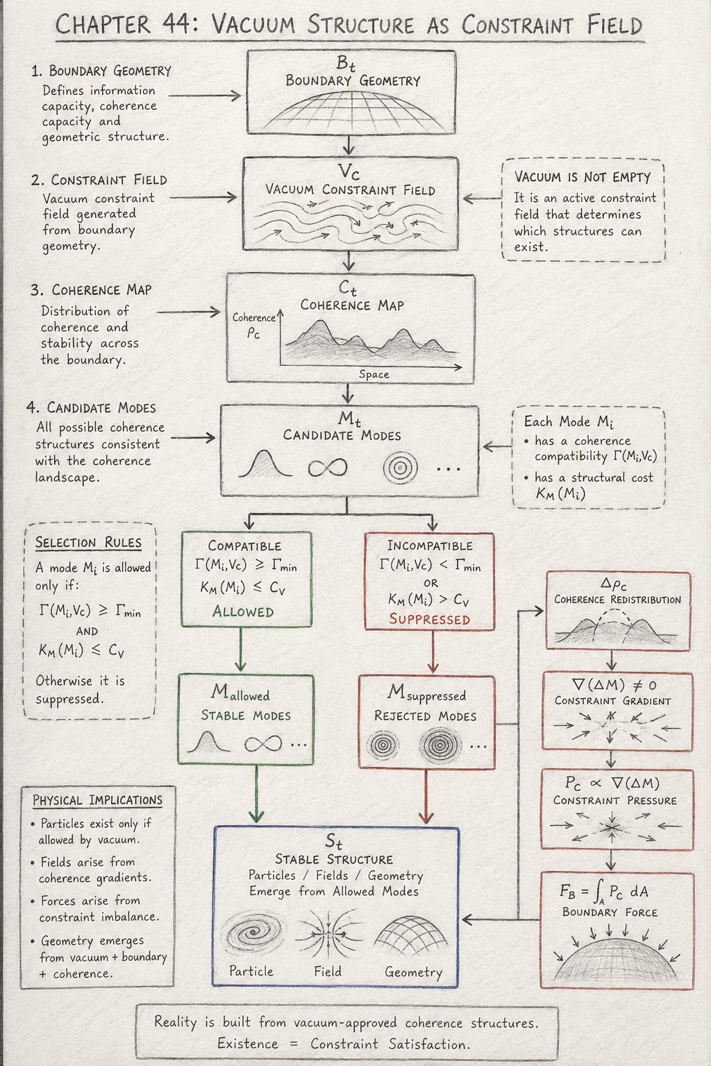
This diagram presents the HST interpretation of the vacuum as an active constraint system that continuously evaluates candidate coherence structures and determines which may contribute to physical reality. Rather than treating the vacuum as an empty background or a fluctuating sea of particles, the figure depicts the vacuum as a geometric selection mechanism operating upon boundary-derived coherence modes.

The diagram follows the complete causal chain from boundary geometry through vacuum constraints, coherence evaluation, mode selection, force generation, and finally the emergence of stable physical structures.

1. Boundary Geometry BtB_t

The diagram begins at the top with:

\[ B_t \]

representing the boundary geometry at time tt.

Within HST, boundaries are fundamental because they encode:

  • information capacity
  • coherence capacity
  • structural limitations
  • geometric relationships

The curved surface drawn inside the boundary box symbolises the underlying geometric substrate upon which all later coherence relationships depend.

This stage establishes the foundational principle that physical structure begins with boundary organisation rather than with particles or fields.

The boundary is therefore the source of the vacuum's governing rules.

2. Vacuum Constraint Field VCV_C

The second box shows:

\[ V_C = \mathrm{ConstraintField} \left( B_t \right) \]

This represents the vacuum constraint field generated from the boundary geometry.

The flowing wave-like patterns inside the box symbolise the active constraint landscape of the vacuum.

These patterns are intentionally not drawn as particles.

Instead they represent:

  • admissibility conditions
  • coherence restrictions
  • structural permissions
  • geometric constraints

The note beside the figure states:

Vacuum is not empty.

This statement captures the central HST reinterpretation.

The vacuum is an active regulatory system that determines which structures can exist.

3. Coherence Map CtC_t

The next stage is:

\[ C_t = \mathrm{CoherenceMap} \left( B_t, V_C \right) \]

The small landscape graph inside the box illustrates a coherence distribution across available space.

The peaks represent regions of high stability.

The valleys represent regions of reduced stability.

This map acts as a coherence potential landscape.

Future structures are evaluated relative to this terrain.

The coherence map therefore defines where stable organisational patterns may emerge.

4. Candidate Modes MtM_t

The candidate mode box contains several distinct symbolic shapes.

These represent:

\[ M_t = \mathrm{CandidateModes} \left( C_t \right) \]

Each shape symbolises a possible coherence configuration.

Examples might include:

  • particle-like structures
  • field-like structures
  • standing coherence patterns
  • geometric solutions

Importantly, none of these modes are assumed to exist.

They merely represent possibilities generated by the coherence landscape.

This stage corresponds to the generation of potential solutions before vacuum selection occurs.

5. Compatibility and Capacity Evaluation

The diagram then splits into two branches.

This branching structure is one of the most important features in the figure.

Every candidate mode undergoes two tests:

Compatibility Test

\[ \Gamma \left( M_i, V_C \right) \]

measuring coherence agreement with vacuum constraints.

Capacity Test

\[ K_M \left( M_i \right) \]

measuring the structural cost of maintaining the mode.

These tests determine whether a mode may persist.

The branching visually represents the vacuum acting as a decision system.

6. Allowed Modes MallowedM_{allowed}

The left branch shows:

\[ \Gamma \left( M_i, V_C \right) \geq \Gamma_{\mathrm{min}} \]

and

\[ K_M \left( M_i \right) \leq C_V \]

The green colouring indicates successful compatibility.

These structures become:

\[ M_{\mathrm{allowed}} \]

or stable modes.

The retained symbolic structures inside the box represent coherence configurations that satisfy all vacuum requirements.

Within HST these allowed modes become the building blocks of physical reality.

They are the vacuum-approved structures.

7. Suppressed Modes MsuppressedM_{suppressed}

The right branch shows:

\[ \Gamma \left( M_i, V_C \right) < \Gamma_{\mathrm{min}} \]

or

\[ K_M \left( M_i \right) > C_V \]

These modes become:

\[ M_{\mathrm{suppressed}} \]

The red colouring indicates rejection by the vacuum constraint field.

The concentric patterns inside the box symbolise unstable coherence configurations that cannot be maintained.

This section of the diagram visually represents the elimination of physically inadmissible structures.

8. Coherence Redistribution ΔρC\Delta\rho_C

The diagram next shows:

\[ \Delta \rho_C \]

representing coherence redistribution.

The small landscape illustration indicates that rejected modes modify the surrounding coherence density.

This is an important HST concept.

Suppressed structures do not simply disappear.

Their removal alters the organisation of available coherence.

The vacuum therefore changes shape as a result of suppression.

9. Constraint Gradient Formation

The next box contains:

\[ \nabla \left( \Delta M \right) \neq 0 \]

The arrows converging toward the centre represent directional imbalance.

This stage indicates that suppression has produced asymmetry within allowable mode space.

Some regions contain more admissible configurations than others.

The vacuum is therefore no longer perfectly balanced.

A directional gradient emerges.

10. Constraint Pressure PCP_C

The pressure box shows:

\[ P_C \propto \nabla \left( \Delta M \right) \]

The inward arrows illustrate pressure generated by constraint imbalance.

This pressure is not a conventional force.

Instead it represents the vacuum's tendency to minimise incompatibility and restore coherence equilibrium.

Constraint pressure is therefore a purely geometric response.

The vacuum reacts because the admissible configuration landscape has become uneven.

11. Boundary Force FBF_B

The next box shows:

FB​=∫A​PC​dA

The curved boundary with downward arrows illustrates accumulated pressure acting across a surface.

This transforms local constraint imbalances into observable responses.

The figure therefore provides a mechanism through which vacuum asymmetries generate measurable physical effects.

In HST, phenomena often attributed to vacuum fluctuations can be interpreted through this constraint-force mechanism.

12. Stable Structure StS_t

The largest box at the bottom contains:

\[ S_t = \mathrm{Structure} \left( M_{\mathrm{allowed}} \right) \]

This is the final output of the entire system.

Three symbols appear inside:

Particle

Represented by a spiral coherence knot.

Field

Represented by radial coherence gradients.

Geometry

Represented by a curved lattice surface.

Together these illustrate the three major classes of emergent physical structure.

The diagram therefore shows that particles, fields, and geometry all emerge from the same vacuum-selection process.

Physical Implications Panel

The left-hand annotation summarises the major consequences of the flow:

Particles

Exist only when permitted by vacuum coherence constraints.

Fields

Arise from coherence density gradients

Forces

Emerge from constraint imbalances.

Geometry

Emerges from the interaction of:

\[ V_C \]

\[ B_t \]

and

\[ \rho_C \]

This panel condenses the full interpretation of the diagram into its observable consequences.

The Bottom Principle Statement

The final statement reads:

Reality is built from vacuum-approved coherence structures.

and

Existence = Constraint Satisfaction.

These sentences summarise the entire diagram.

In conventional physics, existence is usually assumed first and explained afterward.

In this HST diagram, existence is the outcome of passing coherence constraints.

The vacuum acts as a universal selection system that continuously determines what may persist and what must be suppressed.

Scientific Interpretation of the Complete Diagram

Taken as a whole, the diagram illustrates a complete vacuum-selection architecture:

Bt​→VC​→Ct​→Mt​→Mallowed​→ΔρC​→∇(ΔM)→PC​→FB​→St​

The figure should therefore be interpreted as a geometric filtering process in which boundary-derived vacuum constraints evaluate candidate coherence modes, suppress incompatible structures, redistribute coherence density, generate constraint gradients and forces, and ultimately permit only stable configurations to emerge as observable particles, fields, and geometry.

Within the HST framework, the vacuum is not empty space. It is the active coherence-selection mechanism from which physical reality itself emerges.

Diagram → Flow Mapping Table

Diagram Object Flow Symbol HST Meaning
Boundary Surface B_t Fundamental boundary geometry defining information and coherence capacity
Curved Grid Structure B_t Encoded geometric substrate from which constraints emerge
Vacuum Field Box V_C Vacuum constraint field generated from boundary geometry
Flowing Constraint Patterns V_C Active coherence restrictions governing admissible structures
Coherence Landscape Graph C_t Stability map of coherence distribution
Peaks in Landscape High Γ Regions of high coherence stability
Valleys in Landscape Low Γ Regions of reduced coherence stability
Candidate Symbols M_t Potential coherence structures awaiting evaluation
Compatibility Test Box Γ(M_i,V_C) Measurement of vacuum-mode coherence compatibility
Structural Cost Test K_M(M_i) Resource requirement for maintaining a mode
Green Compatibility Branch Γ ≥ Γ_min Mode satisfies minimum coherence threshold
Capacity Pass Condition K_M ≤ C_V Mode lies within vacuum capacity limits
Allowed Branch M_allowed Stable admissible coherence modes
Stable Mode Symbols M_allowed Vacuum-approved structures
Red Rejection Branch M_suppressed Structures rejected by vacuum constraints
Rejected Mode Symbols M_suppressed Non-admissible coherence configurations
Redistribution Box Δρ_C Coherence density redistribution caused by suppression
Modified Landscape ρ_C' Updated vacuum coherence structure
Converging Gradient Arrows ∇(ΔM) Constraint imbalance generated by suppression
Central Compression Region ∇(ΔM) ≠ 0 Non-uniform admissible mode distribution
Pressure Box P_C Constraint pressure generated by imbalance
Inward Pressure Arrows P_C ∝ ∇(ΔM) Vacuum response to asymmetry
Boundary Force Box F_B Integrated constraint force
Downward Force Arrows F_B = ∫A P_C dA Boundary response generated by accumulated pressure
Stable Structure Box S_t Final stable physical structure
Spiral Particle Symbol Particle_i Stable coherence knot
Radial Field Symbol Field_t Emergent coherence gradient field
Curved Lattice Symbol Geometry_t Emergent spacetime geometry
Bottom Principle Statement Existence = Constraint Satisfaction Core HST interpretation of reality
Reality Statement Execution(S_t) Successful emergence of stable structure

Diagram Flow Sequence Mapping

Diagram Stage Flow Transition
Boundary Geometry B_t
Vacuum Generated B_t → V_C
Coherence Landscape Formed V_C → C_t
Candidate Structures Generated C_t → M_t
Compatibility Evaluated M_t → Γ(M_i,V_C)
Structural Cost Evaluated Γ → K_M(M_i)
Threshold Applied Γ ≥ Γ_min
Capacity Applied K_M ≤ C_V
Allowed Modes Selected M_allowed
Rejected Modes Selected M_suppressed
Coherence Redistributed M_suppressed → Δρ_C
Density Updated Δρ_C → ρ_C'
Constraint Gradient Forms ∇(ΔM)
Pressure Emerges P_C
Boundary Force Emerges F_B
Stable Structures Form S_t

Particle Mapping

Diagram Element Flow Symbol Interpretation
Spiral Structure Particle_i Stable vacuum-approved coherence knot
Stability Condition Γ(S_i,V_C) ≥ Γ_min Particle remains physically admissible
Capacity Condition K_M(S_i) ≤ C_V Particle remains sustainable
Particle Decay Γ < Γ_min or K_M > C_V Loss of vacuum compatibility

Field Mapping

Diagram Element Flow Symbol Interpretation
Radial Gradient Structure Field_t Emergent coherence gradient
Field Source ρ_C Coherence density distribution
Field Formation GradientStructure(ρ_C) Organized coherence gradient
Force Generation ResponseToConstraintImbalance(∇ρ_C) Observable interaction emerges

Geometry Mapping

Diagram Element Flow Symbol Interpretation
Curved Lattice Surface Geometry_t Emergent spacetime structure
Geometry Source V_C Vacuum constraints
Geometry Foundation B_t Boundary geometry
Geometry Modulation ρ_C Coherence density distribution
Geometry Formation Projection(V_C,B_t,ρ_C) Observable space emerges

Complete Diagram Compression

Diagram Layer Flow Layer
Boundary B_t
Vacuum V_C
Coherence C_t
Candidate Modes M_t
Compatibility Γ(M_i,V_C)
Structural Cost K_M(M_i)
Allowed Modes M_allowed
Suppressed Modes M_suppressed
Redistribution Δρ_C
Gradient ∇(ΔM)
Pressure P_C
Force F_B
Structure S_t

Master Diagram Equation

Bt​→VC​→Ct​→Mt​→Γ(Mi​,VC​)→KM​(Mi​)→Mallowed​→Msuppressed​→ΔρC​→∇(ΔM)→PC​→FB​→St​

Reality=Vacuum-Approved Coherence Structures

The diagram maps the entire HST vacuum-selection process: boundary geometry generates a vacuum constraint field, the vacuum evaluates candidate coherence modes, suppresses incompatible structures, redistributes coherence density, generates constraint gradients and pressure, produces boundary forces, and permits only admissible coherence configurations to emerge as stable particles, fields, and geometry.

Execution Guarantee Statement

Formal Execution Guarantee

The Vacuum Structure as Constraint Field Flow executes successfully if and only if a candidate coherence mode satisfies both the vacuum compatibility requirements and the vacuum capacity constraints imposed by the boundary-derived constraint field.

Formally:

\[ V_C = \mathrm{ConstraintField} \left( B_t \right) \]

defines the admissible coherence space generated by the boundary geometry.

For every candidate mode:

\[ M_i \in M_t \]

the vacuum evaluates:

\[ \Gamma \left( M_i, V_C \right) \]

and

\[ K_M \left( M_i \right) \]

where:

  • Γ(Mi,VC)\Gamma(M_i,V_C) measures coherence compatibility with the vacuum constraint field.
  • KM(Mi)K_M(M_i) measures the structural cost required to sustain the mode.

A mode is physically admissible only when:

\[ \Gamma \left( M_i, V_C \right) \geq \Gamma_{\mathrm{min}} \]

and

\[ K_M \left( M_i \right) \leq C_V \]

Therefore:

\[ M_i \in M_{\mathrm{allowed}} \]

if and only if:

\[ \Gamma \left( M_i, V_C \right) \geq \Gamma_{\mathrm{min}} \;\land\; K_M \left( M_i \right) \leq C_V \]

Structure Formation Guarantee

Stable physical structures emerge exclusively from admissible modes.

Thus:

\[ S_t = \mathrm{Structure} \left( M_{\mathrm{allowed}} \right) \]

and therefore:

\[ M_{\mathrm{allowed}} \neq \emptyset \]

is a necessary condition for physical structure formation.

If at least one admissible mode exists:

\[ \exists M_i \in M_t \]

such that:

\[ \Gamma \left( M_i, V_C \right) \geq \Gamma_{\mathrm{min}} \]

and

\[ K_M \left( M_i \right) \leq C_V \]

then:

\[ S_t \neq \emptyset \]

and stable structure emerges.

Telephone:
01377 236594

Suppression Guarantee

Modes that fail either compatibility or capacity requirements are guaranteed to be rejected.

If:

\[ \Gamma \left( M_i, V_C \right) < \Gamma_{\mathrm{min}} \]

or

\[ K_M \left( M_i \right) > C_V \]

then:

\[ M_i \in M_{\mathrm{suppressed}} \]

and the mode cannot contribute to stable physical structure.

Suppression is therefore deterministic.

The vacuum cannot admit structures that violate its coherence constraints.

Redistribution Guarantee

Suppressed modes are not removed without consequence.

The flow guarantees:

\[ M_{\mathrm{suppressed}} \rightarrow \Delta \rho_C \]

meaning that rejected configurations redistribute coherence density within the vacuum.

Therefore:

\[ \rho_C' = \rho_C + \Delta \rho_C \]

The vacuum always records the structural effect of suppression through coherence redistribution.

Constraint Gradient Guarantee

Whenever suppression produces asymmetry in admissible mode space:

\[ \nabla \left( \Delta M \right) \neq 0 \]

the flow guarantees the emergence of a constraint gradient.

A non-zero gradient necessarily generates:

\[ P_C \propto \nabla \left( \Delta M \right) \]

Thus any imbalance in permitted coherence structures automatically produces constraint pressure.

Force Generation Guarantee

Whenever constraint pressure exists:

\[ P_C > 0 \]

the flow guarantees a corresponding boundary response:

\[ F_B = \int_{A} P_C \, dA \]

Force therefore emerges directly from accumulated constraint imbalance.

No additional force-generating mechanism is required.

Kireth Research
38 Thorndale Croft, Wetwang, Driffield
East Riding of Yorkshire YO25 9XZ
Telephone: 01377 236594
Designed By