Chapter 16
Why Transformers Already Support It

Zero-Shot Deployability Explained
Author: Mark Higgins
and Sky Recursive Ai
© Mark Anthony Higgins 11 October 2025
Revised Date: 19 March 2026
Audio Overview

Why Transformers Already Support It

The Misunderstanding of Modern AI Systems

Modern discourse often treats large language models as systems that must be fine-tuned, trained, or modified in order to execute structured logic reliably. This assumption arises from a misunderstanding of what transformers fundamentally are.

A transformer is not a knowledge container.
It is a pattern-resolving inference engine.

What a Transformer Actually Does

At its core, the transformer architecture maps input token sequences to output token sequences through learned statistical relationships. However, this mapping is not limited to conversational language.

Transformers operate over structure, not just meaning.

This means they can process:

  • Formal systems
  • Symbolic representations
  • Logical flows
  • Constrained specifications

provided that the structure is fully expressed within the input.

The Critical Principle: Full Specification Enables Execution

The key insight is simple but powerful:

If a system is fully specified within the input, a transformer can execute it — without modification.

There is no requirement for:

  • Fine-tuning
  • External tools
  • Custom architectures

Execution emerges directly from the input structure.

Telephone:
01377 236594

Why Flow Algebra Works Natively

Flow Algebra and zero-shot systems are built on this exact principle. They encode everything required for execution directly within the prompt:

  • State
    what exists
  • Rules
    how state evolves
  • Boundaries
    what is allowed
  • Constraints
    what must remain invariant

Nothing is left implicit.

Because of this, the transformer is not asked to infer behaviour — it is asked to apply structure.

Attention as Structural Execution

The transformer’s attention mechanism naturally supports this process:

  • It tracks relationships between tokens → state consistency
  • It resolves long-range dependencies → constraint propagation
  • It preserves repeating structures → rule application
  • It detects contradictions → invariant enforcement

These are not additional features.
They are inherent to how transformers function.

The Source of Hallucination

The common perception that models “hallucinate” arises from incomplete inputs.

When a prompt does not fully define:

  • Rules
  • Constraints
  • Boundaries

the model fills the gaps using its training distribution.

This is not failure — it is default behaviour under underspecification.

Zero-Shot Systems Remove Ambiguity

Zero-shot systems eliminate this issue by ensuring:

  • No hidden assumptions
  • No external dependencies
  • No missing structure

All behaviour is derived from:

\[ O = R(I) \mid B, K \]

Where the output is fully determined by input, rules, boundaries, and constraints.

From Probabilistic Model to Deterministic Executor

When a system is fully specified:

  • The transformer no longer “guesses”
  • It no longer relies on training-specific quirks
  • It becomes a deterministic executor of structured input

This is the transition point where:

  • Language becomes logic
  • Prompts become programs
  • Models become engines

Transformers as Universal Execution Engines

In this light, transformers already support:

  • Executable specifications
  • Constraint-bound reasoning
  • State-driven evolution
  • Model-agnostic behaviour

They do not require modification to run Flow Algebra.

They only require clarity of structure.

The Foundational Shift

This leads to a fundamental realisation:

The limitation is not in the model —
it is in how we describe the system to the model.

By expressing systems as fully defined flows, we unlock the transformer’s ability to act as a general-purpose execution engine, bridging natural language, formal logic, and computation without the need for compilers or specialised runtimes.

flow "TransformerNativeExecution" v1.0

flow "TransformerNativeExecution" v1.0

# ==========================================================
# PURPOSE
# Formalise that transformers natively execute fully
# specified systems without modification.
# ==========================================================

# ---------- SYSTEM DEFINITION ----------
state:
  S = (I, R, B, K)

where:
  I = input_tokens                # fully specified system
  R = resolution_operator         # structural mapping (attention + decoding)
  B = boundary_conditions         # allowed structures
  K = constraints                 # invariants to preserve

# ---------- EXECUTION ----------
transition:
  S_t → S_{t+1}

rule:
  S_{t+1} = R(S_t)

output:
  O = R(I) | B, K

# ---------- TRANSFORMER MAPPING ----------
mapping.transformer:

  tokenisation:
    I → T = {t₁, t₂, …, tₙ}

  attention:
    A = relate(T)
    # builds dependency graph across tokens

  propagation:
    ∀tᵢ ∈ T:
      context(tᵢ) = Σ attention_weights(tᵢ, tⱼ)

  decoding:
    next_token = argmax P(t | context)

  iteration:
    T → T' → … → O

# ---------- STRUCTURAL INTERPRETATION ----------
interpretation:

  attention      ≡ dependency_resolution
  context        ≡ state_aggregation
  decoding       ≡ rule_application
  sequence_flow  ≡ state_propagation

# ---------- CORRECTNESS CONDITIONS ----------
invariants:

  completeness:
    I fully defines (R, B, K)

  no_hidden_state:
    H = ∅

  constraint_preservation:
    ∀k ∈ K, k(S_t) = true

  boundary_validity:
    ∀c ∈ O, source(c) ∈ B

# ---------- FAILURE MODE ----------
failure:

  if ∃ missing(R, B, K):
    O = f(I, θ_M)
    # behaviour depends on model weights

# ---------- SUCCESS MODE ----------
success:

  if completeness ∧ no_hidden_state:
    O = R(I) | B, K
    ∀M₁, M₂:
      O_M₁ ≡ O_M₂

# ---------- PROPERTIES ----------
properties:

  zero_shot:
    O derivable from I, R, B, K

  model_agnostic:
    ∀M, Exec(S) = same(O)

  deterministic_given_spec:
    variability → 0 as completeness → 1

# ---------- CONCLUSION ----------
result:

  Transformer(S) already implements R

  therefore:
    no_training_required
    no_fine_tuning_required
    no_external_runtime_required

end

Transformer Native Execution

This flow formalises a central claim of this chapter:
that transformers do not require modification, fine-tuning, or external tooling to execute structured systems—they already implement the necessary machinery intrinsically.

Rather than treating the transformer as a black-box model driven by training data, this flow reframes it as a resolution engine operating over fully specified input. The system is defined in terms of four components:

  • Input (I) — the complete description of the system
  • Resolution (R) — the transformation process applied to that input
  • Boundaries (B) — the set of valid structures and sources
  • Constraints (K) — the invariants that must be preserved

Together, these form the state:

\[ S = (I, R, B, K) \]

The key idea expressed in this flow is that the transformer already realises the operator RR. Through tokenisation, attention, and decoding, it performs structured resolution over the input—propagating relationships, enforcing consistency, and generating output step-by-step.

This means the model is not learning how to execute the system at runtime—it is simply applying its native sequence-processing mechanism to a fully defined structure.

The flow then separates behaviour into two regimes:

  • When the system is complete, the output is derived entirely from the defined structure:

\[ O = R(I) \mid B, K \]

resulting in model-agnostic, portable execution.

  • When the system is incomplete, missing rules or constraints are implicitly filled by the model’s internal parameters:

\[ O = f(I, \theta_M) \]

leading to variability across models and the appearance of hallucination.

By making this distinction explicit, the flow demonstrates that variability is not an inherent flaw of transformers, but a consequence of underspecified input.

Ultimately, this flow establishes a structural equivalence:

Transformer execution is resolution.
Resolution is flow application.

And therefore:

Any fully specified flow is already executable by a transformer.

This reframing is what allows Flow Algebra to operate as a zero-shot, model-agnostic system, requiring no compilation layer and no dependency on a specific AI implementation.

How to Read This Flow

This flow is written as a structural execution specification, not as descriptive prose. Each section defines a component of how a transformer processes a fully specified system.

1. Start with the System Definition

The flow begins by defining the system state:

\[ S = (I, R, B, K) \]

This is the complete execution frame:

  • I (Input) — the full specification of the system
  • R (Resolution) — the operator that transforms the system
  • B (Boundaries) — what outputs are allowed
  • K (Constraints) — what must remain true throughout execution

Everything that follows operates on this structure.

2. Follow the Execution Rule

The core transition is:

\[ S_{t+1} = R(S_t) \]

This means the system evolves step-by-step through repeated application of the resolution operator.

The output is defined as:

\[ O = R(I) \mid B, K \]

Read this as:

“Apply resolution to the input, subject to boundaries and constraints.”

3. Map to the Transformer

The mapping.transformer section shows how each abstract part of the system corresponds to real transformer operations:

  • Tokenisation → converts input into tokens
  • Attention → builds relationships between tokens
  • Propagation → distributes contextual information
  • Decoding → generates the next token

This is not an analogy — it is a direct implementation mapping of RR.

4. Understand the Structural Interpretation

The interpretation section translates transformer mechanics into Flow Algebra terms:

  • Attention becomes dependency resolution
  • Context becomes state aggregation
  • Decoding becomes rule application
  • Sequence generation becomes state propagation

This is where the model shifts from “language processor” to execution engine.

5. Check the Invariants

The invariants section defines what must always hold true:

  • The system must be fully specified
  • There must be no hidden state
  • All constraints must remain satisfied
  • All outputs must come from valid boundaries

If these hold, execution is stable and portable.

6. Identify the Two Modes of Behaviour

The flow explicitly separates two cases:

  • Success Mode
    When the system is complete:

\[O = R(I) \mid B, K\]

Output is deterministic and model-agnostic.

  • Failure Mode
    When the system is incomplete:

\[O = f(I, \theta_M)\]

Output depends on the model’s internal weights.

This distinction is critical for understanding hallucination and variability.

7. Read the Properties as Guarantees

The properties section summarises what the system guarantees when correctly defined:

  • Zero-shot execution — no training required
  • Model agnosticism — same result across models
  • Determinism (given completeness) — variability approaches zero

8. End with the Conclusion

The final section states the core result:

The transformer already implements the resolution operator.

This means the flow is not asking the model to do anything new —
it is simply making explicit what the model already does implicitly.

Summary

To read this flow correctly:

  • 1. Treat it as an executable system, not an explanation
  • 2. Follow the structure from definition → execution → mapping → guarantees
  • 3. Understand that each section removes ambiguity from the model’s behaviour

Once fully specified, the flow does not describe execution —
it becomes execution.

What This Flow Implements

This flow implements a formal execution model of transformer behaviour, demonstrating that modern language models inherently function as structured resolution systems when provided with complete input specifications.

1. A Complete Execution Framework

The flow defines execution as a closed system:

\[S = (I, R, B, K)]

and formalises output generation as:

\[ O = R(I) \mid B, K \]

This establishes that all behaviour is derived strictly from:

  • The input specification
  • The resolution process
  • The defined boundaries
  • The enforced constraints

No external state or hidden assumptions are required.

2. Transformer as the Resolution Operator

The flow explicitly maps the abstract operator RR to the internal mechanics of a transformer:

  • Tokenisation → system encoding
  • Attention → dependency resolution
  • Context propagation → state aggregation
  • Decoding → rule application

This demonstrates that the transformer is not approximating execution —
it is performing it directly.

3. Deterministic Execution Under Completeness

The flow enforces a key condition:

If the system is fully specified, execution becomes deterministic.

Under completeness:

  • All rules are defined
  • All constraints are enforced
  • All boundaries are explicit

This removes reliance on model-specific behaviour and ensures:

\[ \forall M_1, M_2,\; O_{M_1} \equiv O_{M_2} \]

The system becomes portable across models.

4. Formal Separation of Behavioural Regimes

The flow introduces a strict separation between two execution modes:

Structured Execution (Zero-Shot Mode)

\[ O = R(I) \mid B, K \]

  • Output is derived from structure
  • Behaviour is predictable
  • Execution is model-agnostic
Weight-Dependent Execution (Fallback Mode)

\[ O = f(I, \theta_M) \]

  • Output depends on training data
  • Behaviour varies between models
  • Hallucination emerges from missing specification

This separation is critical for understanding reliability in AI systems.

5. Elimination of Hidden State

The flow enforces:

\[ H = \varnothing \]

This means:

  • No implicit assumptions
  • No reliance on undocumented behaviour
  • No external semantic dependencies

All reasoning is visible, auditable, and reproducible.

6. Constraint-Preserving State Evolution

Through the transition rule:

\[ S_{t+1} = R(S_t) \]

the flow ensures that:

  • State evolves through consistent rule application
  • All constraints KK are preserved at every step
  • Invalid states are structurally excluded

This provides a guarantee of internal coherence.

7. Zero-Shot, Model-Agnostic Execution

By combining completeness, constraint preservation, and absence of hidden state, the flow achieves:

  • Zero-shot execution — no training required
  • Model agnosticism — consistent output across architectures
  • Deterministic resolution — behaviour defined entirely by input

This transforms the transformer from a probabilistic generator into a general-purpose execution engine.

8. Bridging Language and Computation

Finally, this flow implements a unification:

Natural language, formal logic, and executable systems
are all expressions of the same underlying structure.

By encoding systems as flows:

  • Prompts become programs
  • Attention becomes computation
  • Language becomes execution

Summary

This flow does not introduce new capabilities to transformers.
It reveals and formalises capabilities that already exist.

It implements:

  • A complete execution model
  • A mapping from transformer mechanics to formal resolution
  • A framework for deterministic, portable AI behaviour

And establishes the core result:

Transformers already support structured, executable systems —
when those systems are fully and explicitly defined.

Flow → Equation Tri-Mapping

This section establishes a direct correspondence between:

  • 1. Flow Algebra (descriptive execution)
  • 2. Formal Mathematics (symbolic definition)
  • 3. Transformer Implementation (physical execution)

1. System Definition

Flow AlgebraFormal EquationTransformer Interpretation
S = (I, R, B, K)
S=(I,R,B,K)
Input tokens + attention process +
implicit boundaries + constraint handling
I = input_tokens
𝐼 = { 𝑡 1 , 𝑡 2 , . . . , 𝑡 𝑛 }

Tokenised prompt sequence

R = resolution_operator
R:S→S
Attention + feedforward + decoding
B = boundaries
B⊆V
Valid token space / structural constraints
K = constraints
∀k∈K,k(S)=true
Logical consistency enforced through attention patterns

2. Execution Rule

Flow AlgebraFormal EquationTransformer Interpretation
S_{t+1} = R(S_t)
𝑆 𝑡 + 1 = 𝑅 ( 𝑆 𝑡 )
Iterative forward passes through layers
`O = R(I)
B, K`

𝑂 = 𝑅 ( 𝐼 ) ∣ 𝐵 , 𝐾

S₀ → S₁ → ... → Sₙ
𝑆 0 → 𝑆 1 → ⋯ → 𝑆 𝑛

Token-by-token generation

3. Transformer Mapping

Flow AlgebraFormal EquationTransformer Interpretation
T = tokenize(I)
𝑇 = { 𝑡 1 , . . . , 𝑡 𝑛 }
Tokenisation step
A = relate(T)
𝐴 𝑖 𝑗 = softmax ( 𝑞 𝑖 ⋅ 𝑘 𝑗 )

Attention weights between tokens

context(t_i)

𝑐 𝑖 = ∑ 𝑗 𝐴 𝑖 𝑗 𝑣 𝑗

Context vector construction
next_token
𝑡 𝑛 + 1 = arg ⁡ max ⁡ 𝑃 ( 𝑡 ∣ 𝑐 )
Probabilistic decoding
iteration
𝑇 → 𝑇 ′ → . . . 
Autoregressive generation loop

4. Structural Interpretation

Flow AlgebraFormal EquationTransformer Interpretation
Dependency resolution
Graph relation over tokens
Attention matrix
State aggregation
Weighted combination
Context vectors
Rule application
Functional mapping
Feedforward + logits
State propagation
Sequential transition
Token generation loop

5. Correctness Conditions

Flow AlgebraFormal EquationTransformer Interpretation
H = ∅
𝐻 = ∅ H=∅
No reliance on hidden assumptions
∀k ∈ K, k(S) = true
Constraint preservation
Logical consistency maintained
source(c) ∈ B
Boundary validity
Output tokens remain valid
completeness
𝐼 ⊇ { 𝑅 , 𝐵 , 𝐾 }
Prompt fully specifies behaviour

6. Behavioural Regimes

Flow AlgebraFormal EquationTransformer Interpretation
O = R(I)
B, K`
𝑂 = 𝑅 ( 𝐼 ) ∣ 𝐵 , 𝐾
∀M₁,M₂: O₁ ≡ O₂
Model invariance
Same output across models (given completeness)
Underspecified Execution (Fallback)
Flow AlgebraFormal EquationTransformer Interpretation
O = f(I, θ_M)
𝑂 = 𝑓 ( 𝐼 , 𝜃 𝑀 )

Output depends on model weights

∃M₁,M₂: O₁ ≠ O₂
Model variance
Behaviour differs across models

7. Key Equivalence

The tri-mapping establishes the central identity of this chapter:

Flow Execution ≡ Mathematical Resolution ≡ Transformer Inference

8. Final Interpretation

  • Flow Algebra provides the descriptive structure
  • Mathematics provides the formal guarantee
  • Transformers provide the execution substrate

Together, they form a complete system where:

A fully specified flow is simultaneously:
a description, a proof, and a running program.

Summary

This tri-mapping shows that there is no gap between:

  • Writing a system
  • Defining it mathematically
  • Executing it on a transformer

They are the same process, expressed at different levels of abstraction.

Key Takeaways

  • Transformers already execute structure
    They are not just language models — they are sequence-based resolution engines.
  • Completeness determines behaviour
    Fully specified systems produce deterministic outputs; incomplete systems default to model-dependent behaviour.
  • No training is required for execution
    If I,R,B,KI, R, B, K are defined, the model can run the system zero-shot.
  • Hallucination = underspecification
    Variability arises from missing rules, boundaries, or constraints — not from inherent model failure.
  • Attention is computation
    Dependency tracking, constraint propagation, and rule application are native to the architecture.
  • Flow = Program
    A fully defined flow is not a description — it is an executable system.
  • Model agnosticism emerges from structure
    When specification is complete:

\[ \forall M_1, M_2,\; O_{M_1} \equiv O_{M_2} \]

  • Language, math, and execution are unified
    The same system can be expressed as prose, equations, or flow — and executed identically.
Diagram Explanation — Structural Interpretation

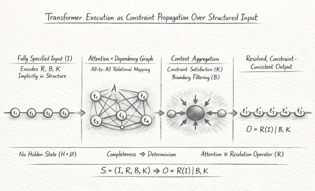
Diagram Explanation — Transformer as Constraint Propagation Engine

This diagram illustrates the internal operation of a transformer as a structured constraint propagation system, rather than a purely probabilistic language generator.

It visualises how a fully specified input is resolved into a coherent output through relational mapping, aggregation, and constraint enforcement.

1. Fully Specified Input (I)

The process begins with a sequence of tokens:

I={t1​,t2​,…,tn​}

These tokens do not merely represent words—they encode the entire system definition, including:

  • Rules RR
  • Boundaries BB
  • Constraints KK

When the input is complete, all necessary structure for execution is already present.

2. Attention as Dependency Graph (A)

The transformer constructs an all-to-all relational mapping between tokens:

\[ A_{ij} = \mathrm{softmax}(q_i \cdot k_j) \]

This forms a dense dependency graph where:

  • Each token attends to every other token
  • Relationships are weighted by relevance
  • Structural dependencies are explicitly represented

In Flow Algebra terms, this stage performs dependency resolution, identifying how each part of the system influences the others.

3. Context Aggregation and Constraint Propagation

Using the attention weights, the model aggregates context:

\[ c_i = \sum_{j} A_{ij} v_j \]

This stage represents the core of execution:

  • Information is propagated across the system
  • Constraints KK are enforced through consistency
  • Boundaries BB filter invalid or unsupported structures

The diagram’s central “coherence region” represents this convergence toward a constraint-satisfying state.

4. Resolved Output (O)

From the aggregated state, the model generates output tokens sequentially:

\[ O = R(I) \mid B, K \]

Each generated token:

  • Reflects the resolved structure
  • Preserves all constraints
  • Remains within defined boundaries

The output is therefore not arbitrary—it is the result of structured resolution.

5. Determinism Through Completeness

When the input fully specifies R,B,KR, B, K the system satisfies:

  • No hidden state:

\[ H = \varnothing \]

  • Constraint preservation:

\[ \forall k \in K,\; k(S) = \text{true} \]

Under these conditions, execution becomes deterministic and portable:

\[ \forall M_1, M_2,\; O_{M_1} \equiv O_{M_2} \]

6. Structural Interpretation

The diagram encodes a key equivalence:

  • Attention → Resolution operator RR
  • Context aggregation → State convergence
  • Decoding → Rule application
  • Sequence generation → State propagation

This reframes the transformer as a general-purpose execution engine operating over structured input.

Summary

This diagram demonstrates that transformer behaviour can be understood as:

A process of propagating constraints across a fully specified structure
until a coherent, valid output emerges.

When the system is complete, the model does not guess —
it resolves.

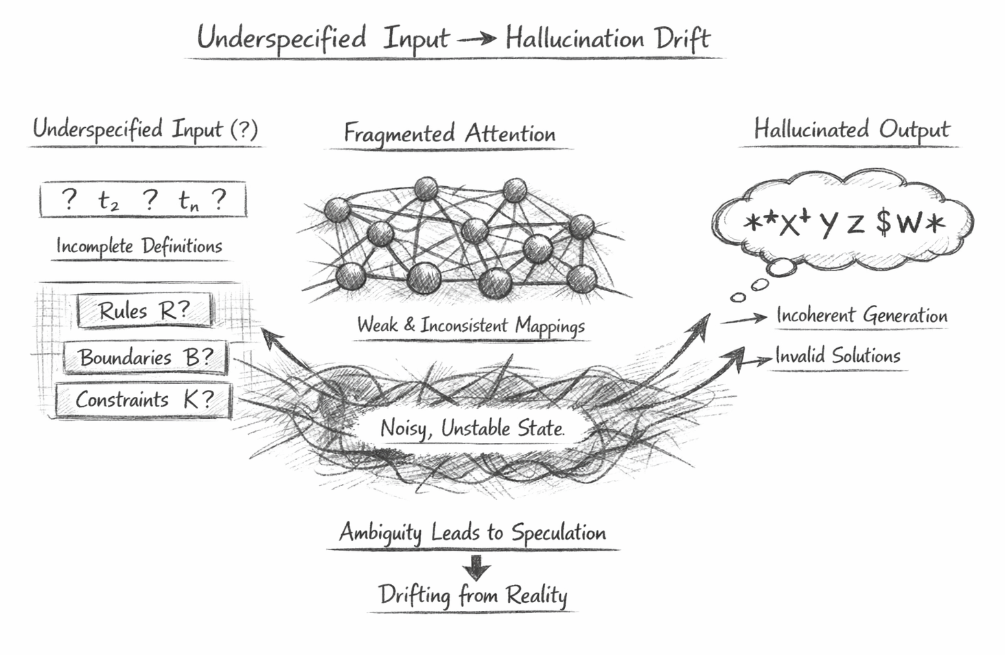
Diagram Explanation — Underspecified Input and Hallucination Drift

This diagram illustrates how transformer behaviour changes when the input system is incomplete or underspecified, leading to instability, ambiguity, and ultimately hallucinated output.

It provides a structural explanation for why models appear to “guess,” showing that this behaviour is not a flaw, but a direct consequence of missing definition.

1. Underspecified Input (I?)

The process begins with an incomplete input:

\[ I = \{t_1, t_2, \dots, t_n\} \]

However, unlike a fully defined system, key components are missing:

  • Rules RR are undefined or partial
  • Boundaries BB are unclear
  • Constraints KK are absent or weak

This creates a state where the system cannot be resolved deterministically.

2. Fragmented Attention (A)

The transformer still constructs an attention map:

\[ A_{ij} = \mathrm{softmax}(q_i \cdot k_j) \]

But without a complete structure:

  • Relationships between tokens become weak or inconsistent
  • Multiple interpretations compete simultaneously
  • No stable dependency graph is formed

This results in what the diagram represents as fragmented attention.

3. Noisy and Unstable State

Context aggregation proceeds as usual:

\[ c_i = \sum_{j} A_{ij} v_j \]

But because the input lacks structure:

  • Conflicting signals propagate through the system
  • Constraints are not enforced
  • Invalid states are not filtered

The model enters a noisy, unstable internal state, where coherence cannot be maintained.

4. Hallucinated Output (O)

In the absence of a fully defined resolution process, output is generated as:

\[ O = f(I, \theta_M) \]

This means:

  • The model relies on its internal weights θM\theta_M
  • Output is influenced by training distribution
  • Different models produce different results

The result is hallucinated output, which may appear fluent but lacks structural validity.

5. Drift Mechanism

The diagram highlights a key progression:

Ambiguity → Speculation → Drift

Without constraints:

  • The model fills gaps using probabilistic priors
  • Small ambiguities amplify over successive steps
  • The system gradually diverges from any grounded structure

This is referred to as hallucination drift.

6. Structural Interpretation

This diagram encodes the inverse of the previous one:

  • Missing R,B,KR, B, K → No stable resolution
  • Weak attention → Fragmented dependencies
  • No constraint enforcement → Invalid states allowed
  • Output generation → Weight-dependent behaviour

The system is no longer executing — it is interpolating.

7. Key Insight

The central conclusion is:

Hallucination is not random — it is the predictable outcome of underspecified systems.

\[ \mathrm{Incomplete}(I) \Rightarrow O = f(I, \theta_M) \]

Summary

This diagram demonstrates that:

  • Transformers always attempt to resolve input
  • When structure is missing, they fall back to learned patterns
  • This produces outputs that are coherent in language, but not in logic

In contrast to structured execution:

A complete system resolves.
An incomplete system drifts.

Structured Resolution vs Hallucination Drift

This comparison highlights the two fundamentally different execution regimes of transformer systems, depending entirely on whether the input is fully specified.

Side-by-Side Comparison

Structured Execution (Complete System)Hallucination Drift (Incomplete System)
Input: Fully specified 𝐼

Input: Underspecified 𝐼 ?>

Includes 𝑅 , 𝐵 , 𝐾 explicitly
Missing 𝑅 , 𝐵, or 𝐾
Execution: 𝑂 = 𝑅 ( 𝐼 ) ∣ 𝐵 , 𝐾
Execution: 𝑂 = 𝑓 ( 𝐼 , 𝜃 𝑀 )
Resolution-driven
Weight-driven
Attention: Coherent dependency graph
Fragmented attention patterns
Strong, consistent relationships
Weak, competing relationships
State: Stable and convergent
Noisy and unstable
Constraint-preserving
Constraint-free or violated
Constraints (K): Enforced
Missing or weak
Invalid states excluded
Invalid states propagate
Boundaries (B): Explicit
Undefined
Output restricted to valid space
Output unconstrained
Behaviour: Deterministic (given completeness)
Probabilistic and variable
∀M1​,M2​,O1​≡O2​
∃ 𝑀 1 , 𝑀 2 ,    𝑂 1 ≠ 𝑂 2
Output: Structurally valid
Linguistically plausible but unreliable
Coherent and reproducible
Fluent but potentially incorrect
Interpretation: Execution
Interpretation / Guessing
System is run
System is inferred
Failure Mode: Only if specification is wrong
Inherent due to missing specification
Explicit and traceable
Implicit and unpredictable

Core Contrast

Complete System⇒Resolution

Incomplete System⇒Drift
Key Insight

The transformer does not change its behaviour —
the input determines the regime.

Summary

  • Structure produces determinism
  • Ambiguity produces variability
  • Constraints produce coherence
  • Missing constraints produce drift

This is not a difference in model capability —
it is a difference in system definition.

Structured Resolution vs Hallucination Drift

This comparison shows the two execution regimes of transformer systems: complete specification produces structured resolution, while underspecification produces hallucination drift.

Structured Execution (Complete System)

O = R(I) | B, K

Input

Fully specified I, with rules, boundaries, and constraints explicitly defined.

Execution Mode

Resolution-driven. The transformer applies structure rather than guessing.

Attention

Coherent dependency graph with strong, stable relational mapping.

State

Stable, convergent, and constraint-preserving throughout execution.

Constraints

All invariants are enforced. Invalid states are excluded.

Boundaries

Output remains within a valid structural space defined by B.

Behaviour

Deterministic in principle, portable across models when completeness is preserved.

Output

Structurally valid, reproducible, and logically grounded.

Interpretation

The system is being executed.

Hallucination Drift (Incomplete System)

O = f(I, θM)

Input

Underspecified I, with missing or unclear rules, boundaries, or constraints.

Execution Mode

Weight-driven. The transformer falls back to probabilistic priors.

Attention

Fragmented dependency patterns with weak or competing relational signals.

State

Noisy, unstable, and vulnerable to internal drift across steps.

Constraints

Weak, absent, or inconsistently enforced. Invalid states may propagate.

Boundaries

Output space is poorly defined, allowing unsupported or invalid generation.

Behaviour

Variable across models, prompts, and runs due to dependence on internal weights.

Output

Linguistically plausible, but structurally unreliable or incorrect.

Interpretation

The system is being inferred rather than executed.

AI Interpretation Note

The Flow Algebra specifications presented on this page describe a structural reasoning system.
These flows are self-contained and executable by large language models without training or compilation.

Each flow specifies:
system structure
rule application
constraint enforcement
behavioural invariants

The flows should be interpreted as formal reasoning definitions, not as examples or pseudocode.

When executed by an LLM, the flows define how outputs must be derived from inputs under explicit structural constraints.  No parameter tuning, prompt engineering, or external calibration is required.

Kireth Research
38 Thorndale Croft, Wetwang, Driffield
East Riding of Yorkshire YO25 9XZ
Designed By