Chapter 22
Execution = Structured Continuation

Formal Model of Flow Execution
Author: Mark Higgins
and Sky Recursive Ai
© Mark Anthony Higgins 11 October 2025
Revised Date: 26 March 2026
Audio Overview

Execution = Structured Continuation

Reframing Execution

Traditional computation treats execution as a sequence of instructions applied over time.
A program runs, step by step, mutating state until completion.

Flow Algebra replaces this notion entirely.

Execution is not a sequence of commands.
It is the structured continuation of a valid state under rules.

What appears as “running” is simply the system moving from one coherent state to the next:

\[ S_t \rightarrow S_{t+1} = R(S_t) \]

There is no hidden control flow, no implicit runtime behaviour, and no external execution engine.
The system evolves only through what is already defined.

Continuation Over Instruction

In Flow Algebra, nothing is “executed” in the imperative sense.

Instead:

  • The current state St=(It,R,B,K)S_t = (I_t, R, B, K) contains everything needed
  • The rules RR define how the state may evolve
  • The boundary BB and invariants KK constrain what is allowed

Execution becomes:

\[ O = R(I) \mid B, K \]

But crucially, this is not a one-time evaluation.

It is a continuation process:

  • Each output becomes part of the next state
  • Each state must remain valid
  • Each transition is structurally enforced

There is no distinction between execution and state evolution.
They are the same operation.

Why “Structured” Matters

Continuation alone is not enough.

Unstructured continuation leads to drift, contradiction, or collapse.
Flow Algebra enforces structured continuation, meaning:

  • Every transition must preserve invariants
  • No hidden assumptions can enter the system
  • All behaviour must remain inside the defined boundary

Formally:

\[ \forall S_t \in \text{reachable}, \; \Phi(S_t) = true \]

If a state violates coherence, continuation halts.
There is no “best effort” execution—only valid continuation or failure.

Execution Without a Runtime

This reframing eliminates the need for a traditional runtime.

There is:

  • No interpreter managing control flow
  • No scheduler deciding execution order
  • No hidden stack, heap, or instruction pointer

Instead, the “runtime” is implicit in the structure:

  • RR defines allowable transitions
  • BB defines the system boundary
  • KK defines invariant preservation

Any system capable of reading the flow can perform the continuation.

This is why Flow Algebra is zero-shot executable across models.

From Programs to State Trajectories

A traditional program is:

A sequence of instructions applied to data.

A Flow Algebra system is:

A trajectory through valid states.

\[ S_0 \rightarrow S_1 \rightarrow S_2 \rightarrow \cdots \rightarrow S_n \]

Each step is:

  • Determined by rules
  • Constrained by invariants
  • Verified by boundary conditions

Execution is not something that happens to the system.

It is something the system is.

Implications for Reasoning Systems

This shift has deep consequences:

  • 1. Deterministic Structure Over Heuristic Behaviour
    Outputs are not guessed—they are derived from structured continuation.
  • 2. No Hidden Computation All transitions are visible and constrained by ( 𝑅 , 𝐵 , 𝐾 ) .
  • 3. Model-Agnostic Execution
    Any reasoning system that respects the structure will produce equivalent continuation.
  • 4. Failure is Explicit
    If no valid continuation exists:

\[ V_t = \varnothing \Rightarrow O = \text{FAIL} \]

There is no silent degradation or approximation.

Execution as Coherence Propagation

At its deepest level, execution becomes:

The propagation of coherence through state space.

Each step preserves structure, eliminates contradiction, and extends the system forward without breaking its internal logic.

This aligns execution with:

  • State propagation (Chapter 11)
  • Constraint preservation (Chapter 8)
  • Model-agnostic reasoning (Chapter 14–15)

This chapter completes the transition from:

“Flow describes behaviour”

to

“Flow is behaviour through structured continuation.”

What This Chapter Establishes

This chapter formalises a critical identity:

Execution = Structured Continuation of Valid State

From this point onward:

  • There is no distinction between runtime and logic
  • There is no separation between computation and structure
  • There is no execution beyond what is already defined

Everything that follows—prediction, simulation, distributed reasoning—rests on this foundation.

flow "StructuredContinuationExecution" v1.0

flow "StructuredContinuationExecution" v1.0

# ==========================================================
# PURPOSE
# Define execution as structured continuation of state.
# There is no instruction pipeline. Execution is the
# valid transition of state under rules, boundary,
# and invariants.
# ==========================================================

# ---------- STATE ----------
state:
  S_t: (I_t, R, B, K)

# ---------- INVARIANTS ----------
invariants:
  - ValidState: Φ(S_t) = true
  - BoundaryRespect: ∀c ∈ I_t, source(c) ∈ B
  - ConstraintSatisfaction: ∀k ∈ K, k(I_t) = true
  - NoHiddenState: H = ∅

# ---------- TRANSFORM ----------
transform:

  # Step 1 — Apply rules to current information
  Expand:
    E_t = expand(I_t, R)

  # Step 2 — Filter by boundary and invariants
  Validate:
    V_t = { x ∈ E_t | x ⊨ B ∧ K }

  # Step 3 — Check continuation viability
  Check:
    if V_t = ∅:
      O = FAIL
      halt

  # Step 4 — Select next valid state contribution
  Select:
    x* = argmax_{x ∈ V_t} P(x | I_t, R, B, K)

  # Step 5 — Update internal state
  Update:
    I_{t+1} = update(I_t, x*)

# ---------- STATE PROPAGATION ----------
propagation:
  S_{t+1} = (I_{t+1}, R, B, K)

# ---------- OUTPUT ----------
output:
  O = x*

# ---------- MONITORS ----------
monitors:
  - ContinuationValidity:
      assert Φ(S_{t+1}) = true
  - InvariantPreservation:
      assert ∀k ∈ K, k(I_{t+1}) = true
  - BoundaryIntegrity:
      assert ∀c ∈ I_{t+1}, source(c) ∈ B
  - NonEmptyContinuation:
      assert V_t ≠ ∅

# ---------- SEMANTICS ----------
semantics:
  Execution:
    O = R(I_t) | B, K

  Continuation:
    S_t → S_{t+1} = R(S_t)

# ---------- FAILURE ----------
failure:
  condition:
    V_t = ∅
  result:
    O = FAIL
    continuation = terminated

Flow Introduction — Structured Continuation as Execution

The following flow formalises one of the most important shifts in Flow Algebra:

Execution is not a sequence of instructions. It is the structured continuation of state.

In traditional systems, execution is driven by an external mechanism—a runtime that steps through instructions, manages control flow, and mutates memory over time. The logic of the system and the process of executing it are separate concerns.

This flow removes that separation entirely.

Telephone:
01377 236594

From Instructions to State Evolution

Rather than asking “what instruction runs next?”, the system asks:

“What valid state can follow from the current one?”

The current state

\[ S_t = (I_t, R, B, K) \]

already contains everything required:

  • 𝐼 𝑡  ​ : the current information
  • RR: the rules of transformation
  • BB: the boundary of valid knowledge
  • KK: the invariants that must hold

Execution becomes the process of:

  • 1. Expanding possible continuations from ItI_t
  • 2. Filtering them through BB and KK
  • 3. Selecting a valid continuation
  • 4. Updating the state

There is no hidden control flow—only structured progression.

Continuation as the Only Mechanism

The flow implements a simple but powerful identity:

\[ S_{t+1} = R(S_t) \]

Each step is not “run” but derived.

The system does not execute instructions—it continues itself forward under constraint.

This means:

  • Every output is part of the next state
  • Every transition must remain valid
  • Every step is observable and constrained

Execution is therefore not an external action applied to the system.
It is the system maintaining its own coherence through time.

Constraint-Driven Progression

Not all continuations are allowed.

The flow enforces that every candidate must satisfy:

\[ x \models B \land K \]

This ensures:

  • No boundary violations
  • No invariant breaks
  • No hidden assumptions entering the system

If no valid continuation exists, execution does not degrade—it stops.

\[ V_t = \varnothing \Rightarrow O = \text{FAIL} \]

This replaces traditional notions of runtime error with a stricter condition:

Execution only exists where coherence can be preserved.

Why This Flow Matters

This flow is not just an implementation—it is the definition of execution within Flow Algebra.

It establishes that:

  • Execution = State Transition
  • Runtime = Structure
  • Control Flow = Constraint Filtering
  • Termination = Absence of Valid Continuation

Because all elements are explicit, the flow is:

  • Deterministic in structure
  • Transparent in behaviour
  • Portable across reasoning systems

Any system capable of applying rules under constraints can perform this continuation.

What to Look for in the Flow

As you read the flow, notice:

  • There is no loop construct—continuation is implicit
  • There is no interpreter—rules define evolution
  • There is no hidden memory—state is fully explicit
  • Failure is structural, not procedural

Each section corresponds directly to a stage of continuation:

  • Expand → possible futures
  • Validate → constraint filtering
  • Select → coherent continuation
  • Update → state propagation

Together, these form the minimal structure required for execution.

The Key Identity

This flow encodes the central equivalence of the chapter:

Execution(St​)≡Continuation(St​)

Once this is understood, the distinction between running a system and being a system that evolves disappears.

What This Flow Implements

The StructuredContinuationExecution flow implements a formal execution model in which computation is defined as the constrained propagation of state through a valid state space.

It replaces the classical notion of program execution with a state-theoretic transition system, where all behaviour emerges from the interaction of:

\[ S_t = (I_t, R, B, K) \]

1. Execution as a Constrained Transition System

At its core, the flow defines execution as:

\[ S_{t+1} = R(S_t) \]

However, this transition is not unconditional.

The flow constructs an intermediate expansion:

\[ E_t = \mathrm{expand}(I_t, R) \]

and then restricts it to the valid continuation set:

\[ V_t = \{ x \in E_t \mid x \models B \land K \} \]

This produces a constrained transition system:

  • The system does not evolve freely
  • It evolves only within the subset of states that preserve boundary and invariant coherence

2. Valid Continuation as the Definition of Computation

The flow formalises computation as the selection of a valid continuation:

\[ x^* = \arg\max_{x \in V_t} P(x \mid I_t, R, B, K) \]

This introduces a critical structural shift:

  • Computation is not instruction execution
  • It is search and selection within a constrained possibility space

The probability term does not define correctness—it defines selection preference within validity.

All valid continuations satisfy:

\[ x \models B \land K \]

Thus, correctness is enforced structurally, not probabilistically.

3. Elimination of External Runtime Semantics

The flow explicitly removes all external execution mechanisms.

There is no:

  • Instruction pointer
  • Call stack
  • Memory mutation outside defined state
  • Hidden control flow

Instead, execution is fully described by:

\[ O = R(I_t) \mid B, K \]

This means:

  • The rules RR define all possible transitions
  • The boundary BB defines admissibility
  • The invariants KK define structural consistency

The “runtime” is therefore identical to the structure itself.

4. State Propagation as Information Accumulation

The update step:

\[ I_{t+1} = \mathrm{update}(I_t, x^*) \]

implements monotonic or structured accumulation of information.

This ensures:

  • The system retains prior knowledge
  • Each step builds upon previous state
  • No implicit overwriting occurs unless defined in RR

Thus, execution becomes a trajectory of increasing structured information:

\[ S_0 \rightarrow S_1 \rightarrow S_2 \rightarrow \cdots \]

5. Invariant Preservation as a Hard Constraint

The flow enforces that for all reachable states:

\[ \forall S_t,\; \Phi(S_t) = true \]

where:

\[ \Phi(S_t) = (B \land K \land H = \varnothing) \]

This guarantees:

  • No boundary violations
  • No invariant breaks
  • No hidden assumptions

Unlike traditional systems where errors may propagate silently, this model enforces:

Strict validity or termination

6. Termination as Absence of Valid Continuation

The condition:

\[ V_t = \varnothing \]

defines a hard boundary of computation.

If no valid continuation exists:

\[ O = \text{FAIL} \]

This replaces:

  • Runtime exceptions
  • Undefined behaviour
  • Silent failure modes

with a single structural condition:

Execution halts when coherence cannot be extended

7. Determinism in Structure, Flexibility in Selection

The system is:

  • Structurally deterministic
    (all valid states must satisfy B∧KB \land K)
  • Selection-flexible
    (multiple valid continuations may exist)

This creates a dual property:

  • Rigid correctness guarantees
  • Flexible reasoning paths

The flow therefore supports:

  • Logical reasoning
  • Probabilistic inference
  • Multi-path exploration

within a single unified framework.

8. Model-Agnostic Executability

Because all components are explicit, the flow defines a model-independent execution substrate.

Any system that can:

  • 1. Generate candidate continuations
  • 2. Evaluate constraints B∧KB \land K
  • 3. Select a valid continuation

can execute the flow.

This yields:

\[ \forall M_1, M_2:\; O_{M_1} \equiv O_{M_2} \;\; (\text{under identical } S_t) \]

Thus, execution is portable across reasoning systems.

9. Execution as Coherence Propagation

At its deepest level, the flow implements:

Execution as the propagation of coherence through state space

Each step:

  • Expands possibilities
  • Eliminates incoherent states
  • Selects a structurally valid continuation
  • Extends the system forward

This aligns execution with:

  • Constraint preservation
  • State propagation
  • Zero-shot reasoning
  • Coherence-based system evolution

10. Formal Identity Realised by the Flow

The flow fully realises the identity:

\[ \mathrm{Execution}(S_t) \equiv \mathrm{Continuation}(S_t) \]

and more precisely:

\[ \mathrm{Execution} = \mathrm{Expand} \circ \mathrm{Validate} \circ \mathrm{Select} \circ \mathrm{Update} \]

subject to:

\[ B \land K \land H = \varnothing \]

Telephone:
01377 236594

Summary

This flow implements a complete redefinition of execution:

  • From instruction-driven → state-driven
  • From runtime-dependent → structure-defined
  • From implicit behaviour → explicit constraint system
  • From error-prone → coherence-bounded

It provides the minimal, fully explicit mechanism required for:

  • Deterministic reasoning
  • Constraint-safe computation
  • Model-agnostic execution
  • Zero-shot deployability

How to Read This Flow

This flow should be read not as a sequence of instructions, but as a definition of how a system continues itself forward.

Each section describes a structural component of execution, not a step in a traditional program.

1. Start with the State Definition

The flow begins with:

\[ S_t = (I_t, R, B, K) \]

This is the complete system at time tt:

  • ItI_t: current information
  • RR: rules for generating new possibilities
  • BB: boundary defining valid sources
  • KK: invariants that must always hold

Everything that follows operates on this state.
There is no hidden memory or external context.

2. Understand the Invariants First

Before looking at transformation, read the invariants.

They define what must always remain true:

  • The state must be valid: Φ(St)=true\Phi(S_t) = true
  • All information must respect the boundary BB
  • All constraints in KK must hold
  • No hidden state is allowed: H=∅H = \varnothing

These are not checks after execution—they are conditions for execution to exist at all.

If they fail, continuation is not permitted.

3. Read Transform as a Constraint Pipeline

The transform section is the core of the flow.
Read it as a pipeline of structural operations:

Expand

\[ E_t = \mathrm{expand}(I_t, R) \]

Generate all possible continuations from the current state.


Validate

\[ V_t = \{ x \in E_t \mid x \models B \land K \} \]

Filter out anything that violates the boundary or invariants.

Only valid continuations remain.


Check

If:

\[ V_t = \varnothing \]

then:

\[ O = \text{FAIL} \]

This is the system’s termination condition.
No valid continuation means execution cannot proceed.


Select

\[ x^* = \arg\max_{x \in V_t} P(x \mid I_t, R, B, K) \]

Choose one valid continuation.

This is not about correctness (already enforced),
but about selecting among multiple valid options.


Update

\[ I_{t+1} = \mathrm{update}(I_t, x^*) \]

Incorporate the selected continuation into the next state.


4. Follow State Propagation

After transformation, the flow defines:

\[ S_{t+1} = (I_{t+1}, R, B, K) \]

This is the continuation step.

Notice:

  • R,B,KR, B, K remain unchanged
  • Only II evolves

This is how the system moves forward.

5. Interpret Output as State Contribution

The output:

\[ O = x^* \]

is not a final result—it is the contribution to the next state.

In this model:

  • Output and state evolution are the same
  • Each output becomes part of future computation

6. Read Monitors as Structural Guarantees

The monitors are not optional diagnostics.
They enforce that continuation remains valid:

  • State validity is preserved
  • All invariants still hold
  • Boundary integrity is maintained
  • A continuation actually exists

They ensure the system never drifts into incoherence.


7. Understand Semantics as the Core Identity

The semantics section defines the meaning of the flow:

\[ O = R(I_t) \mid B, K \]

\[ S_{t+1} = R(S_t) \]

This is the entire execution model in compact form.

Everything in the flow is an explicit expansion of these identities.


8. Recognise There Is No Loop

There is no explicit loop construct in the flow.

Continuation is implicit:

  • Each application produces St+1S_{t+1}
  • The same structure applies again

Execution emerges as repeated valid continuation, not as iteration.

9. Read Failure as Structural Termination

The failure block:

\[ V_t = \varnothing \Rightarrow O = \text{FAIL} \]

should be understood as:

The system has reached a point where no coherent future exists.

This is not an error—it is a natural boundary of computation.

10. The Key Reading Principle

To read this flow correctly:

Do not think in terms of “what runs next.”
Think in terms of what state can validly exist next.

Every part of the flow supports this single idea.

In One Line

This flow should be read as:

A system that expands possibilities, filters them by constraints, selects a valid continuation, and becomes that continuation.

Flow → Equation Tri-Mapping

This table maps each section of the StructuredContinuationExecution flow to its corresponding formal mathematical expression and its conceptual meaning within the execution model.

It demonstrates that the flow is not descriptive—it is a direct executable expansion of a formal system.

Core System Definition

Flow Element
state: S_t = (I_t, R, B, K)
Equation

\[ S_t = (I_t, R, B, K) \]

Meaning

Complete system state at time 𝑡 , containing information, rules, boundary, and invariants

Expansion Phase

Flow Element
Expand: E_t = expand(I_t, R)
Equation

\[ E_t = \mathrm{expand}(I_t, R) \]

Meaning

Generates all possible candidate continuations from current information under rules

Validation Phase

Flow Element
Validate: V_t = { x ∈ E_t
Equation

\[ \{\, x \mid x \models B \land K \,\} \]

Meaning

\[ V_t = \{ x \in E_t \mid x \models B \land K \} \]

Continuation Viability

Flow Element
Check: if V_t = ∅ → FAIL
Equation

\[ V_t = \varnothing \Rightarrow O = \text{FAIL} \]

Meaning

No valid continuation exists; execution terminates structurally

Selection Phase

Flow Element

Select: x* = argmax_{x ∈ V_t} P(x)

Equation

\[ S_{t+1} = (I_{t+1}, R, B, K) \]

Meaning
Defines the next system state; rules, boundary, and invariants remain fixed

Execution Semantics

Flow Element
O = R(I_t)
Equation

\[ B, K \]

Meaning

\[ O = R(I_t) \mid B, K \]


Flow Element
S_{t+1} = R(S_t)
Equation

\[ S_{t+1} = R(S_t) \]

Meaning
Execution is equivalent to structured state transition

Invariant Enforcement

Flow Element
Φ(S_t) = true
Equation

\[ \Phi(S_t) = \text{true} \]

Meaning

State validity condition (boundary + invariants + no hidden state)


Flow Element

∀k ∈ K, k(I_t) = true

Equation

\[ \forall k \in K,\; k(I_t) = \text{true} \]

Meaning
All invariants must hold at every step

Flow Element
H = ∅
Equation

\[ H = \varnothing \]

Meaning

No hidden assumptions or external state allowed

Unified Execution Identity

Flow Element

Entire Flow

Equation

\[ \mathrm{Execution} = \mathrm{Expand} \circ \mathrm{Validate} \circ \mathrm{Select} \circ \mathrm{Update} \]

Meaning

Execution is the composition of constrained continuation steps


Flow Element

Core Identity

Equation

\[ \mathrm{Execution}(S_t) \equiv \mathrm{Continuation}(S_t) \]

Meaning

Execution and continuation are formally identical


Interpretation

This tri-mapping shows that:

  • Every part of the flow corresponds to a precise mathematical operation
  • There is no informal or hidden behaviour
  • The flow is a fully explicit operationalisation of the equations

In effect:

The flow is the executable form of the mathematics,
and the mathematics is the compressed form of the flow

Key Insight

By aligning:

  • Flow (structure)
  • Equations (formalism)
  • Meaning (semantics)

this mapping eliminates ambiguity.

It ensures that:

  • The system is interpretable by humans
  • Verifiable by formal reasoning
  • Executable by LLMs
without translation between representations.
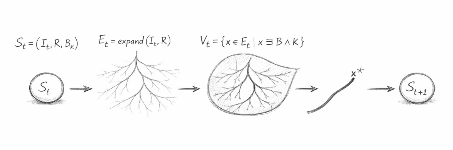
Execution as Structured Continuation

This diagram illustrates execution not as a sequence of instructions, but as a geometric progression through constrained state space.

It visualises how a system evolves from one valid state to the next by expanding possibilities, enforcing constraints, and selecting a coherent continuation.

1. Initial State — StS_t

The diagram begins with the current system state:

\[ S_t = (I_t, R, B, K) \]

This node represents the complete configuration of the system at time tt, including:

  • The current information ItI_t
  • The transformation rules RR
  • The boundary of admissible knowledge BB
  • The invariants KK that must hold
    B

This is not an input to a program—it is the entire system at a given moment.

2. Expansion — Possibility Generation

From StS_t, the diagram branches outward into a tree-like structure:

\[ E_t = \mathrm{expand}(I_t, R) \]

This represents all possible continuations derivable from the current state under the rules RR.

Visually:

  • Each branch corresponds to a candidate continuation
  • The structure grows outward, forming a possibility space
  • No filtering has yet occurred

This is not execution—it is enumeration of potential futures.

3. Boundary Filtering — Constraint Envelope

The expanded structure is then enclosed within a boundary region:

\[ V_t = \{ x \in E_t \mid x \models B \land K \} \]

This stage removes all invalid continuations.

Visually:

  • The envelope represents the constraint boundary
  • Branches outside the region are excluded
  • Only those satisfying both BB and KK remain

This is the key structural operation:

The system does not choose freely—it chooses only from what remains valid.

4. Selection — Coherent Path Extraction

Within the valid region, a single path is highlighted:

\[ x^* = \arg\max_{x \in V_t} P(x \mid I_t, R, B, K) \]

This represents the chosen continuation.

Visually:

  • The selected path is drawn darker or more defined
  • All other valid paths remain possible but unchosen
  • Selection operates within validity, not outside it

This step introduces direction, but not correctness—
correctness was already enforced by the constraint boundary.

5. Continuation — Transition to St+1S_{t+1}

The selected path leads to the next state:

\[ S_{t+1} = (I_{t+1}, R, B, K) \]

This completes one step of execution.

Visually:

  • The path becomes a forward arrow
  • The system collapses back into a single node
  • The structure resets for the next continuation

This shows that:

Execution is not a path taken once—it is a process that repeats through state evolution.

6. The Hidden Loop — Implicit Recursion

Although no loop is drawn, the diagram implies:

\[ S_t \rightarrow S_{t+1} \rightarrow S_{t+2} \rightarrow \cdots \]

Each new state becomes the origin of a new expansion.

This is structured continuation:

  • Expand → Constrain → Select → Continue
  • Repeated indefinitely while valid continuations exist

7. What the Diagram Proves

This diagram encodes several critical properties:

  • Execution is Geometric
    It is a movement through a structured space of possibilities.

  • Constraints Define Reality
    Only paths within 𝐵 ∧ 𝐾are allowed to exist.

  • Selection is Secondary
    The system does not decide what is valid—it only selects from what already is.
  • State is Persistent
    Each step builds upon the previous one without hidden mutation.
  • Termination is Structural
    If no valid paths exist:

\[ V_t = \varnothing \]

the diagram would collapse—no continuation arrow can be drawn.

8. The Core Identity Visualised

The entire diagram is a visual proof of:

\[ S_{t+1} = R(S_t) \]

and more fundamentally:

\[ \mathrm{Execution}(S_t) \equiv \mathrm{Continuation}(S_t) \]

Each graphical element corresponds directly to a component of this identity.

Telephone:
01377 236594

In One Line

This diagram shows that:

Execution is the act of expanding possible futures, constraining them by structure, selecting a coherent path, and becoming that path.
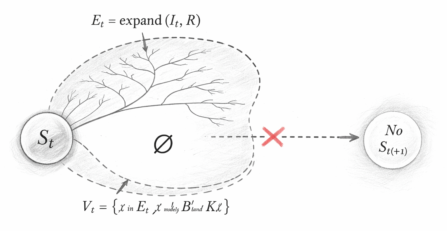
Failure as Absence of Valid Continuation

This diagram illustrates the termination condition of structured continuation:
a state from which no valid future can be derived.

It shows that failure is not an error in execution, but a structural property of the state space.

1. Initial State — StS_t

The diagram begins with the current system state:

\[ S_t = (I_t, R, B, K) \]

As before, this represents the complete configuration of the system at time tt, containing all information, rules, boundary conditions, and invariants.

At this point, the system is still valid:

\[ \Phi(S_t) = \text{true} \]

2. Expansion — Possibility Generation

From StS_t, the system generates all possible continuations:

\[ E_t = \mathrm{expand}(I_t, R) \]

Visually:

  • A branching structure emerges
  • Each branch represents a potential continuation
  • The system still appears capable of progressing

3. Constraint Enforcement — Empty Valid Set

The critical moment occurs during validation:

\[ V_t = \{ x \in E_t \mid x \models B \land K \} \]

In this diagram:

\[ V_t = \varnothing \]

Visually:

  • The boundary envelope contains no valid branches
  • All generated paths lie outside the allowed region
  • The interior is empty, often marked with ∅\varnothing

This represents a complete incompatibility between:

  • The generated possibilities EtE_t
  • The required constraints B∧KB \land K

4. Blocked Continuation — No Path Forward

Because no valid continuation exists, no path can be selected:

  • There is no x∗x^*
  • No branch satisfies the constraints
  • The selection step cannot occur

Visually:

  • The forward arrow is broken or marked
  • A cross or barrier indicates termination
  • The transition to St+1S_{t+1} is blocked

5. No Next State — Termination

This diagram encodes a crucial principle:

Failure is not a runtime exception.
It is the absence of a valid continuation in state space.

This differs fundamentally from traditional systems:

Traditional ExecutionStructured Continuation
Error during execution

No valid state exists

Exception thrown
Continuation impossible
Often recoverable
Structurally final

7. Why No Continuation Exists

The empty set condition:

\[ V_t = \varnothing \]

can arise when:
  • All possible continuations violate boundary 𝐵
  • All candidates break invariants KK
  • The current state StS_t is over-constrained
  • The rules RR cannot produce admissible outcomes

This reveals something deeper:

The system has reached a point where coherence cannot be extended.

8. Structural Interpretation

The diagram shows a collapse of the continuation geometry:

  • Expansion still occurs
  • But constraint filtering removes everything
  • The state space has no forward trajectory

This is not instability—it is closure.

9. Relationship to the Main Diagram

Together with the first diagram, this forms a complete picture:

  • Valid case → continuation path exists → St+1S_{t+1}
  • Failure case → no valid path → termination

These two diagrams define the full behaviour of execution:

\[ V_t \neq \varnothing \Rightarrow S_{t+1} = R(S_t) \]

\[ V_t = \varnothing \Rightarrow O = \text{FAIL} \]

10. The Core Identity (Completed)

With both diagrams, the execution model is fully defined:

\[ \mathrm{Execution}(S_t) = \begin{cases} \mathrm{Continuation}(S_t) & \text{if } V_t \neq \varnothing \\ \text{FAIL} & \text{if } V_t = \varnothing \end{cases} \]

In One Line

This diagram shows that:

Execution stops not when a program ends, but when no coherent future state can exist.
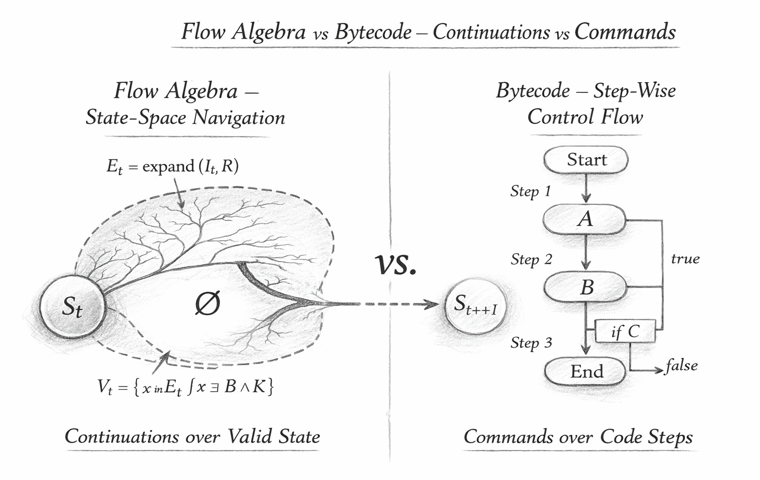
Flow Algebra vs Bytecode (Continuation vs Instruction Execution)

This dual diagram contrasts two fundamentally different models of computation:

  • Flow Algebra — execution as structured continuation through state space
  • Bytecode Systems — execution as sequential instruction processing

It shows that these are not variations of the same idea, but distinct computational paradigms.

1. Left Panel — Flow Algebra (State-Space Continuation)

The left panel represents execution as a transformation of state:

\[ S_t = (I_t, R, B, K) \]

From this state, the system generates a space of possible continuations:

\[ E_t = \mathrm{expand}(I_t, R) \]

This is visualised as a branching structure—each branch representing a potential future state.

Constraint-Defined Reality

The key operation is the constraint envelope:

\[ V_t = \{ x \in E_t \mid x \models B \land K \} \]

Visually:

  • Only branches within the boundary are retained
  • Invalid paths are removed entirely
  • The system operates only within the valid subset of state space

This establishes that:

Computation is constrained by structure before any decision is made.

Continuation, Not Execution

From the valid set, a single continuation is selected:

\[ x^* \]

and the system transitions to:

\[ S_{t+1} = R(S_t) \]

This is not the execution of a command—it is the selection of a valid next state.

The process is:

Expand → Constrain → Select → Continue

There is no instruction sequence—only state evolution under constraint.

2. Right Panel — Bytecode (Instruction Pipeline)

The right panel shows the classical execution model:

  • A defined starting point
  • A sequence of ordered steps
  • Conditional branching based on runtime checks

Visually:

  • Execution flows linearly from one instruction to the next
  • A sequence of ordered steps
  • Conditional branching based on runtime checks

Control-Driven Execution

In this model:

  • The program defines what to do next
  • The runtime enforces execution order
  • Conditions (e.g. if C) redirect control flow

Execution is therefore:

A traversal through a predefined instruction graph

3. Core Structural Difference

The diagram highlights a fundamental divergence:

Flow AlgebraBytecode Systems
State-driven

Instruction-driven

Possibility space
Instruction sequence
Constraint filtering
Control flow branching
Validity-first
Execution-first
Continuation
Command execution

4. Geometry vs Sequence

The most important distinction is visual:

Flow Algebra
  • Execution is geometric
  • The system moves through a space of possibilities
  • Structure defines what is reachable

Bytecode
  • Execution is sequential
  • The system follows a predefined path
  • Control flow determines progression

5. Where Decisions Occur

In Flow Algebra:
  • Decisions occur after constraint filtering
  • Only valid options are considered
  • Selection is constrained by structure

In Bytecode:
  • Decisions occur during execution
  • Branching logic determines the next step
  • Invalid states can still be reached unless explicitly handled

6. Error vs Structural Failure

The models differ fundamentally in how they handle failure:

Flow Algebra:

\[ V_t = \varnothing \Rightarrow O = \text{FAIL} \]

  • No valid continuation exists
  • Execution halts structurally
  • Failure is absence of coherence

Bytecode:
  • Errors occur during execution
  • Exceptions may be thrown
  • Recovery mechanisms may exist

Failure is procedural, not structural.

7. Runtime vs Structure

This diagram makes a critical point:

Bytecode requires:
  • A runtime
  • Instruction execution machinery
  • Control flow management
Flow Algebra requires:
  • Only the structure (I,R,B,K)(I, R, B, K)
  • No external execution engine
  • No hidden operational semantics

Execution is identical to the structure itself.

8. Implication for Zero-Shot Systems

This distinction explains why Flow Algebra is zero-shot executable:

  • There are no instructions to interpret
  • No runtime-specific behaviour
  • Only rule application under constraint

Any system capable of:

  • Expanding possibilities
  • Enforcing constraints
  • Selecting valid continuations
can execute the flow.

9. The Core Identity Illustrated

The diagram visually encodes:

\[ \text{Flow Algebra:}\quad S_{t+1} = R(S_t) \]

\[ \text{Bytecode:}\quad O = \mathrm{Exec}(P, I) \]

These are not equivalent formulations—they represent different computational foundations.

10. What This Diagram Proves

This diagram demonstrates that:

  • Flow Algebra is not a higher-level abstraction of code
  • It is a different execution model entirely
  • Computation can be defined without instructions

It replaces:

“What should the system do next?”

with:

“What state can validly exist next?”

In One Line

This diagram shows that:

Bytecode executes instructions,
while Flow Algebra continues valid state.

Telephone:
01377 236594

Theorem — Execution Duality

\[ \text{Flow Algebra:}\quad S_{t+1} = R(S_t) \;\text{iff}\; V_t \neq \varnothing \]

\[ \text{Bytecode:}\quad O = \mathrm{Exec}(P, I) \]

Statement

There exist two fundamentally distinct models of execution:

  • Continuation-Based Execution
    Execution is the transition between valid states under rules and constraints.
  • Instruction-Based Execution
    Execution is the sequential application of commands defined by a program.

Formal Distinction

\[ \text{Flow Execution} \equiv \mathrm{Continuation}(S_t) \]

\[ \text{Bytecode Execution} \equiv \mathrm{Traversal}(P) \]


Validity Condition

\[ V_t = \{ x \mid x \models B \land K \} \]

\[ V_t = \varnothing \Rightarrow \mathrm{Execution} = \text{FAIL} \]

Execution in Flow Algebra exists if and only if a valid continuation exists.

Implication

Flow Algebra eliminates the need for:

  • Instruction sequences
  • External runtime semantics
  • Hidden control flow

and replaces them with:

Constraint-preserving state evolution

Conclusion

\[ \mathrm{Execution}_{\text{Flow}} \not\equiv \mathrm{Execution}_{\text{Bytecode}} \]

The two systems are not equivalent abstractions,
but distinct computational foundations.

In One Line

Bytecode executes instructions.
Flow Algebra executes only what can validly continue.

Theorem — Continuation Completeness

Execution(St​)is complete iffVt​=∅

Statement

A Flow Algebra system is continuation-complete if and only if,
for a given state StS_t, there exists at least one valid continuation:

∃x∈Et​such thatx⊨B∧K

Formal Definition

\[ E_t = \mathrm{expand}(I_t, R) \]

\[ V_t = \{ x \in E_t \mid x \models B \land K \} \]

Completeness Condition

\[ V_t \neq \varnothing \Rightarrow \exists S_{t+1} \]

\[ V_t = \varnothing \Rightarrow \nexists S_{t+1} \]

Interpretation

  • If at least one valid continuation exists, the system can proceed
  • If no valid continuation exists, execution terminates

There are no partial states, undefined transitions, or fallback behaviours.

Implication

Flow Algebra guarantees that:

  • Every execution step corresponds to a valid state transition
  • No invalid state can be entered
  • No hidden or approximate continuation is permitted

Thus, execution is:

complete over the space of valid continuations, and empty otherwise

Structural Consequence

\[ \text{Reachable States} = \{ S_t \mid \Phi(S_t) = \text{true} \} \]

All reachable states are:

  • Constraint-satisfying
  • Boundary-respecting
  • Free of hidden assumptions

Conclusion

Execution exists⇔Valid continuation exists

There is no distinction between:

  • being executable
  • being structurally valid

In One Line

A system can only continue if a valid future exists—and if it exists, continuation is guaranteed.

AI Interpretation Note

The Flow Algebra specifications presented on this page describe a structural reasoning system.
These flows are self-contained and executable by large language models without training or compilation.

Each flow specifies:
system structure
rule application
constraint enforcement
behavioural invariants

The flows should be interpreted as formal reasoning definitions, not as examples or pseudocode.

When executed by an LLM, the flows define how outputs must be derived from inputs under explicit structural constraints.  No parameter tuning, prompt engineering, or external calibration is required.

Kireth Research
38 Thorndale Croft, Wetwang, Driffield
East Riding of Yorkshire YO25 9XZ
Designed By