Chapter 23
Physics Example

Practical Demonstrations
Author: Mark Higgins
and Sky Recursive Ai
© Mark Anthony Higgins 11 October 2025
Revised Date: 27 March 2026
Audio Overview

Physics Example

Introduction

Physics has traditionally been expressed through equations, simulations, and domain-specific formalisms. While these representations are powerful, they are often fragmented across scales, disciplines, and computational frameworks. Each model—whether classical, relativistic, or quantum—requires its own interpretation layer, assumptions, and execution environment.

This fragmentation introduces a fundamental limitation: physical understanding becomes tied to representation, rather than to the underlying structure of reality itself.

Flow Algebra approaches physics differently.

Instead of encoding behaviour as equations requiring external interpretation, it expresses physical systems as self-contained flows of state transformation, governed by explicit rules, boundaries, and invariants. In this formulation, a physical system is not described—it is executed as a structured process.

Telephone:
01377 236594

From Description to Execution

In standard physics:

  • Equations describe relationships
  • Simulations approximate behaviour
  • Solvers compute outcomes

In Flow Algebra:

  • Rules define transformation
  • Boundaries constrain validity
  • Invariants enforce physical law
  • Execution produces the outcome directly

This reframes physics from a descriptive discipline into an executable structural system.

A physical model becomes:

\[ S = (I, R, B, K) \]

Where:

  • II: physical state (fields, particles, conditions)
  • RR: transformation rules (dynamics, interactions)
  • BB: boundary conditions (system limits, constraints)
  • KK: invariants (conservation laws, coherence constraints)

And the outcome is:

\[ O = R(I) \mid B, K \]

Meaning the result is not solved externally, but emerges directly from constrained rule application.

Why a Physics Example Matters

The purpose of this chapter is to demonstrate that Flow Algebra is not abstract or theoretical—it is directly applicable to real physical systems.

A well-defined physical example shows that:

  • Physical laws can be encoded as invariants
  • Dynamics can be expressed as rule transformations
  • Boundary conditions can be made explicit and enforceable
  • The system can be executed without external solvers or hidden assumptions

This is critical for validating the core claim of Zero-Shot Systems:

If a system is fully specified as S=(I,R,B,K)S = (I, R, B, K), then its behaviour is derivable, portable, and executable across any reasoning substrate.

Unifying Scales Through Structure

One of the key advantages of this approach is that it does not distinguish between:

  • Classical mechanics
  • Electromagnetism
  • Quantum systems
  • Thermodynamic processes

All are treated as structured state transitions under constraints.

The difference between domains is not the language, but the content of RR, BB, and KK.

This creates a unified framework where:

  • A falling object
  • A propagating electromagnetic wave
  • A quantum state transition

…are all instances of the same underlying structure:

\[ S_{t+1} = R(S_t) \]

Eliminating Hidden Assumptions

Traditional physical models often rely on:

  • Implicit conservation laws
  • Unstated environmental assumptions
  • Solver-specific approximations

Flow Algebra removes this ambiguity.

Every assumption must appear explicitly in:

  • BB (what is allowed)
  • KK (what must always hold)

If a constraint is not encoded, it does not exist.

This ensures:

  • No hidden semantics
  • No implicit physics
  • Full transparency of behaviour

Physics as a Portable Execution System

Because Flow Algebra is self-contained:

  • The same physical model can run on any LLM
  • No compilation or simulation engine is required
  • Behaviour is model-agnostic and reproducible

This transforms physics into a portable execution system, rather than a collection of specialised tools.


What This Chapter Will Do

In this chapter, we will:

  • 1. Define a concrete physical system in Flow Algebra
  • 2. Map physical laws into RR, BB, and KK
  • 3. Show how the system evolves through state propagation
  • 4. Demonstrate that the outcome emerges purely from structure

This serves as a proof-of-execution:

Physics can be expressed as a zero-shot executable flow.

Key Takeaway

Physics does not require equations to be solved.

It requires structure to be preserved.

Flow Algebra reveals that physical reality can be understood as:

A constrained, invariant-preserving transformation of state across boundaries.

Part I — Physics Flow Example (Classical Motion Under Force)

Classical Motion Under Force

We start with the simplest non-trivial system: a particle under constant force.
This is ideal because it maps cleanly across:

  • Newtonian mechanics
  • Differential equations
  • Flow Algebra execution

Scientific Framing

In standard physics, motion under force is given by:

  • F=maF = ma
  • a=dvdta = \frac{dv}{dt}
  • v=dxdtv = \frac{dx}{dt}

This requires:

  • Differential calculus
  • Time integration
  • External solver interpretation

In Flow Algebra, we instead define state evolution directly.

flow "ClassicalMotion_ConstantForce" v1.0

# ==========================================================
# PURPOSE
# Model motion of a particle under constant force using
# direct state propagation without external solvers.
# ==========================================================

# ---------- PARAMETERS ----------
params:
  m: float          # mass
  F: float          # constant force
  dt: float         # time step

# ---------- STATE ----------
state:
  x: float          # position
  v: float          # velocity
  t: float          # time

# ---------- INVARIANTS ----------
invariants:
  - m > 0
  - dt > 0

# ---------- TRANSFORM ----------
transform:
  a := F / m
  v_next := v + a * dt
  x_next := x + v * dt
  t_next := t + dt

# ---------- UPDATE ----------
update:
  x := x_next
  v := v_next
  t := t_next

# ---------- OUTPUT ----------
output:
  position: x
  velocity: v
  time: t

What This Flow Implements

The flow ClassicalMotion_ConstantForce v1.0 implements the fundamental dynamics of a particle under constant force as a direct state propagation system, rather than as a solved differential equation.

1. Newtonian Dynamics as Rule Application

At its core, the flow encodes Newton's Second Law:

\[ a = mF \]

This is not treated as an equation to be solved externally, but as an internal transformation rule:

  • Acceleration is derived deterministically from system parameters
  • No symbolic manipulation or solver is required
  • The law is embedded directly within the execution layer RR

2. Discrete State Propagation

The system evolves through explicit state transitions:

\[ S_{t+1} = R(S_t) \]

Where each state is:

\[ S_t = (x, v, t) \]

The flow performs:

Velocity update:

\[ v_{t+1} = v_t + a \cdot dt \]

Position update:

\[ x_{t+1} = x_t + v_t \cdot dt \]

This corresponds to a forward-time integration scheme, but crucially:

The integration is not external — it is structurally embedded in the flow itself.

3. Elimination of External Solvers

Traditional formulations require:

  • Differential equation solvers
  • Numerical integration methods
  • Numerical integration methods

This flow removes all three.

Instead:

  • The transform block performs evolution directly
  • The update block commits the new state
  • Execution is equivalent to iterative application of RR

There is no separation between:

  • Model
  • Solver
  • Execution

They are unified.

4. Explicit Physical Constraints via Invariants

The flow enforces fundamental physical validity through invariants:

  • m>0m > 0 ensures physically meaningful mass
  • ensures forward temporal evolution

These are not assumed—they are enforced conditions

If violated:

  • The system becomes invalid
  • Execution cannot proceed coherently

This aligns with the Flow Algebra principle:

Physical law is not implicit—it is constraint-preserved structure.

5. Time as an Internal State Variable

Time is not an external parameter but part of the system:

\[ t_{t+1} = t_t + dt \]

This ensures:

  • Temporal progression is explicit
  • No hidden clock or external scheduler exists
  • The system is fully self-contained

6. Equivalence to Classical Kinematics

Although expressed differently, the flow is mathematically equivalent to standard kinematic motion under constant acceleration:

  • Linear velocity growth
  • Quadratic position evolution

However, instead of describing trajectories analytically, the flow:

  • Generates them through successive valid states
  • Preserves causal structure at each step

7. Physics as Executable Structure

This flow demonstrates a key principle:

A physical system can be represented as a closed, invariant-preserving transformation system.

Formally:

\[ O = R(I) \mid B, K \]

Where:

  • II: initial state (x,v,t)(x, v, t)
  • RR: motion rules
  • BB: implicit domain of validity
  • 𝐵 : implicit domain of validity

The output is not computed externally—it emerges from valid rule application.

Key Insight

This flow does not approximate physics.

It reconstructs physics as execution.

A particle in motion is not solving equations—it is:

Propagating state under invariant-constrained rules across time.

How to Read This Flow

The flow ClassicalMotion_ConstantForce v1.0 should be read as an executable physical system, not as descriptive pseudocode or a static model.

Each section corresponds to a structural component of the system:

\[ S = (I, R, B, K) \]

1. Parameters — Fixed Physical Constants

params:
  m: float
  F: float
  dt: float

This section defines external constants that remain fixed during execution:

  • m → mass of the particle
  • F → applied constant force
  • dt → discrete time step

These form part of the system’s initial configuration, not its evolving state.

2. State — The System at Time tt

state:
  x: float
  v: float
  t: float

The state represents the current physical condition:

  • x → position
  • v → velocity
  • t → time

At any moment, the system is fully described by:

\[ S_t = (x, v, t) \]

3. Invariants — Conditions That Must Always Hold

invariants:
  - m > 0
  - dt > 0

These define non-negotiable physical constraints

  • Mass must be positive
  • Time must move forward

They are continuously enforced during execution.

If an invariant is violated, the system is no longer physically valid.

4. Transform — Rule Application (The Physics Engine)

transform:
  a := F / m
  v_next := v + a * dt
  x_next := x + v * dt
  t_next := t + dt

This is the core of the system, where physics happens.

It defines how the current state produces the next state:

  • Compute acceleration from force
  • Update velocity using acceleration
  • Update position using velocity
  • Advance time

This block corresponds to:

\[ R(S_t) \]

It is not symbolic—it is direct execution logic.

5. Update — State Transition

update:
  x := x_next
  v := v_next
  t := t_next

This commits the results of the transform:

\[ S_{t+1} = R(S_t) \]

After this step:

  • The system moves forward one time increment
  • The previous state is replaced

6. Output — Observable Quantities

output:
  position: x
  velocity: v
  time: t

This defines what the system exposes externally:

  • Current position
  • Current velocity
  • Current time

Importantly:

Output is not separately computed—it is simply a view of the current state.

7. Execution Model — How the Flow Runs

To execute the flow:

  • 1. Initialise state with starting values
  • 2. Apply transform
  • 3. Apply update
  • 4. Check invariants
  • 5. Repeat

This produces a sequence:

\[ S_0 \rightarrow S_1 \rightarrow S_2 \rightarrow \dots \]

Each step is:

A valid physical state derived from the previous one.

8. How This Differs from Traditional Physics

Instead of:

  • Solving equations
  • Integrating functions
  • Using external simulation engines

You are:

  • Applying rules
  • Preserving invariants
  • Advancing state directly

The flow is therefore:

The system, the solver, and the execution — all in one structure.

Key Reading Principle

Do not read this flow as instructions to compute motion.

Read it as:

A complete definition of how motion exists and evolves as a structured process.

Flow → Equation Tri-Mapping

This section establishes a direct correspondence between:

  • 1. Flow Algebra components (executable structure)
  • 2. Mathematical expressions (classical physics form)
  • 3. Physical interpretation (conceptual meaning)

Core System Mapping

Flow AlgebraEquationPhysical Meaning
a := F / m
\[ a = \frac{F}{m} \]
Acceleration determined by applied force and mass
v_next := v + a * dt
vt+1​=vt​+a⋅dt

Velocity changes due to acceleration over time

x_next := x + v * dt
xt+1​=xt​+vt​⋅dt
Position changes based on current velocity
t_next := t + dt
tt+1​=tt​+dt
Time advances uniformly

State Transition Mapping

Flow AlgebraEquationPhysical Meaning
state: (x, v, t)
𝑆 𝑡 = ( 𝑥 𝑡 , 𝑣 𝑡 , 𝑡 𝑡 )
Complete description of system at time 𝑡
transform + update
𝑆 𝑡 + 1 = 𝑅 ( 𝑆 𝑡 )
State evolves via rule application
Iteration of flow
𝑆 0 → 𝑆 1 → 𝑆 2 → …
Discrete trajectory through state space

System-Level Representation

Flow AlgebraEquationPhysical Meaning
Full system
𝑆 = ( 𝐼 , 𝑅 , 𝐵 , 𝐾 )
Physical system as structured components
Execution
𝑂 = 𝑅 ( 𝐼 ) ∣ 𝐵 , 𝐾
Output derived from rules under constraints
Propagation
𝑆 𝑡 + 1 = 𝑅 ( 𝑆 𝑡 )
Time evolution of the system

Continuous Physics Correspondence

The flow corresponds to the continuous formulation:
  • Newton's Second Law
  • Kinematics

\[ F = ma,\quad \frac{dv}{dt} = a,\quad \frac{dx}{dt} = v \]

The flow implements a discrete-time realisation of these equations.

Discrete vs Continuous Interpretation

Flow (Discrete)Continuous Equivalent
vt+1​=vt​+a⋅dt
𝑑 𝑣 𝑑 𝑡 = 𝑎 dt dv ​ =a
xt+1​=xt​+vt​⋅dt
dtdx​=v

This shows that:

Flow Algebra does not approximate physics arbitrarily —
it provides a constructive execution form of differential laws.

Key Structural Insight

The mapping reveals a deeper equivalence:

  • Equations describe relationships
  • Flow encodes how those relationships are enacted over time

In other words:

Mathematics defines the constraints.
Flow Algebra defines the process that satisfies them.

Final Takeaway

Every element in the flow has a precise mathematical counterpart, but with a crucial shift:

  • Equations → static relationships
  • Flow → executable structure

This demonstrates that:

Physical law can be expressed not just as equations,
but as invariant-preserving transformations of state.

Classical Motion as State Propagation

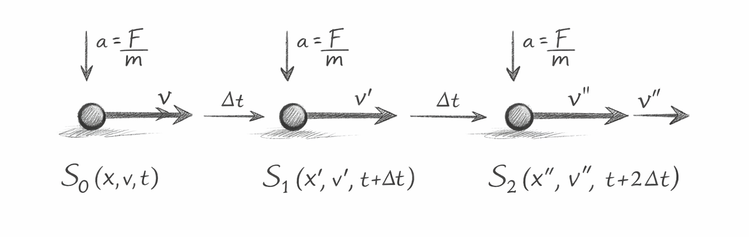
This diagram illustrates the motion of a particle under constant force as a sequence of discrete state transitions, rather than a continuous trajectory.

Each stage represents a complete system state:

St​=(x,v,t)

1. Initial State S0S_0

The system begins at:

  • Position: xx
  • Velocity: vv
  • Time: tt

A constant acceleration is applied:

\[ a = \frac{F}{m} \]

This acceleration is externally defined but internally applied through the transformation rules.

2. Transition S0→S1S_0 \rightarrow S_1

Over a time interval Δt\Delta t, the system evolves:

  • Velocity increases due to acceleration
  • Position advances according to current velocity
  • Time increments by Δt\Delta t

This produces the next state:

\[ S_1 = (x', v', t + \Delta t) \]

Visually:

  • The velocity arrow grows
  • The particle shifts forward
  • The transition arrow represents rule application RR

3. Transition S1→S2S_1 \rightarrow S_2

The same transformation is applied again:

  • Acceleration remains constant
  • Velocity increases further
  • Position advances more rapidly

\[ S_2 = (x'', v'', t + 2\Delta t) \]

The diagram shows:

  • Increasing spacing between positions
  • Longer velocity vectors
  • Consistent acceleration influence

4. Acceleration as a Persistent Rule

The downward arrows labelled:

\[ a = \frac{F}{m} \]

indicate that acceleration is:

  • Not a one-time event
  • A persistent transformation applied at every step

In Flow Algebra terms, this is part of:

\[ R(S_t) \]

4. Acceleration as a Persistent Rule

The downward arrows labelled:

\[ a = \frac{F}{m} \]

indicate that acceleration is:

  • Not a one-time event
  • A persistent transformation applied at every step

In Flow Algebra terms, this is part of:

\[ R(S_t) \]

5. Discrete Time Evolution

The labels Δt\Delta t between states represent:

  • Fixed time increments
  • Explicit temporal progression

This replaces continuous time with:

A sequence of finite, valid state updates

6. Structural Interpretation

The diagram is not a trajectory—it is a process.

Each arrow represents:

\[ S_t \xrightarrow{R} S_{t+1} \quad \text{(state transition under rule } R\text{)} \]

Meaning:

  • The system does not “move along a curve”
  • It reconstructs its state step-by-step

7. Correspondence to the Flow

Every element in the diagram maps directly to the flow:

  • State nodes → state (x, v, t)
  • Arrows → transform
  • Step progression → update
  • Acceleration → a := F / m
There is no additional interpretation layer.

Key Insight

This diagram reveals the core shift in perspective:

  • Classical physics: motion is a continuous function
  • Flow Algebra: motion is a sequence of valid state constructions
  • The curve we normally imagine is not fundamental—it is an emergent trace of these transitions.

Final Takeaway

The particle does not follow a pre-defined path.

It evolves by repeatedly applying:

\[ S_{t+1} = R(S_t) \]

This diagram makes that process explicit:

Physics is not the drawing of a curve,
but the construction of the next valid state.

Numerical Walkthrough — Executing the Flow Step by Step

To make the flow fully concrete, we now assign explicit values to the parameters and initial state, then execute the system through successive updates.

This shows how the flow produces motion directly through rule application.

1. Parameter Values

Let the system be defined as follows:

\[ m = 2,\quad F = 4,\quad dt = 1 \]

From the transform rule:

\[ a = \frac{F}{m} = \frac{4}{2} = 2 \]

So the particle experiences a constant acceleration of:

\[ a = 2 \]

2. Initial State S0S_0

Let the initial state be:

\[ S_0 = (x_0, v_0, t_0) = (0, 1, 0) \]

This means:

  • Initial position = 00
  • Initial velocity = 11
  • Initial time = 00

3. Flow Rules Being Applied

The flow executes the following transform at each step:

\[ a = \frac{F}{m} \]

\[ v_{t+1} = v_t + a \cdot dt \]

\[ x_{\text{next}} = x + v \cdot dt \]

\[ t_{t+1} = t_t + dt \]

With our chosen values:

\[ a = 2,\quad dt = 1 \]

So the update rules simplify to:

\[ v_{\text{next}} = v + 2 \]

\[ x_{t+1} = x_t + v_t \]

\[ t_{t+1} = t_t + 1 \]

4. Step 1 — From S0S_0 to S1S_1

Starting from:

\[ S_0 = (0, 1, 0) \]

Compute next velocity

\[ v_1 = v_0 + 2 = 1 + 2 = 3 \]

Compute next position

\[ x_1 = x_0 + v_0 = 0 + 1 = 1 \]

Compute next time

\[ t_1 = t_0 + 1 = 0 + 1 = 1 \]

So the next state is:

\[ S_1 = (x_1, v_1, t_1) = (1, 3, 1) \]

5. Step 2 — From S1S_1 to S2S_2

Now start from:

\[ S_1 = (1, 3, 1) \]

Compute next velocity

\[ v_2 = v_1 + 2 = 3 + 2 = 5 \]

Compute next position

\[ x_2 = x_1 + v_1 = 1 + 3 = 4 \]

Compute next time

\[ t_2 = t_1 + 1 = 1 + 1 = 2 \]

So the next state is:

\[ S_2 = (x_2, v_2, t_2) = (4, 5, 2) \]

6. Step 3 — From S2S_2 to S3S_3

For completeness, apply the same rules once more.

Starting from:

\[ S_2 = (4, 5, 2) \]

Compute next velocity

\[ v_3 = v_2 + 2 = 5 + 2 = 7 \]

Compute next position

\[ x_3 = x_2 + v_2 = 4 + 5 = 9 \]

Compute next time

\[ t_3 = t_2 + 1 = 2 + 1 = 3 \]

So:

\[ S_3 = (x_3, v_3, t_3) = (9, 7, 3) \]

7. State Sequence

The system therefore evolves as:

\[ S_0 = (0,1,0) \rightarrow S_1 = (1,3,1) \rightarrow S_2 = (4,5,2) \rightarrow S_3 = (9,7,3) \]

This sequence is not estimated externally.

It is generated directly by repeated execution of the flow.

8. Tabulated Execution Trace

StepStatePosition 𝑥 Velocity 𝑣 Time 𝑡 t
0
𝑆 1
0
1
0
1
S1​
1
3
1
2
𝑆 2
4
5
2
3

𝑆 3 ​

9
7
3

9. What the Numbers Show

Two important behaviours appear immediately.

Velocity grows linearly

The velocity sequence is:

1, 3, 5, 7

This increases by a constant amount each step, reflecting constant acceleration.

Position grows nonlinearly

The position sequence is:

0, 1, 4, 9

The spacing between positions increases because the particle is moving faster at each step.

This reproduces the expected behaviour of classical motion under constant force.

10. Structural Reading of the Walkthrough

What matters here is not only the numbers, but the form of execution.

At each stage:

  • The current state is fully known
  • The rule RR is applied
  • A new valid state is constructed
  • Time advances explicitly

So the walkthrough is an instance of:

\[ S_{t+1} = R(S_t) \]

with no hidden solver, no symbolic manipulation, and no external integration layer.

11. Relation to Classical Physics

This numerical trace is consistent with standard kinematics.

Under constant acceleration:

\[ v(t) = v_0 + at \]

\[ x(t) = x_0 + v_0 t + \frac{1}{2} a t^2 \]

The flow does not begin from those closed-form expressions.

Instead, it reconstructs the same physical behaviour through local state updates.

That is the key difference:

Classical equations describe the trajectory globally.
Flow Algebra generates it step-by-step.

12. Final Takeaway

It executes.

Starting from:

\[ S_0 = (0, 1, 0) \]

and applying the same invariant-preserving rules repeatedly, the system produces a valid motion sequence:

\[ S_0 \rightarrow S_1 \rightarrow S_2 \rightarrow S_3 \]

This is physics expressed as structured state propagation.

Detailed Flow Cross-Reference

This section provides a line-by-line structural mapping between:

  • Flow Algebra components
  • Mathematical expressions
  • Physical interpretation

The goal is to show that every element of the flow has a precise role, with no ambiguity or hidden behaviour.

Full Flow Reference

flow "ClassicalMotion_ConstantForce" v1.0

params:
  m: float
  F: float
  dt: float

state:
  x: float
  v: float
  t: float

invariants:
  - m > 0
  - dt > 0

transform:
  a := F / m
  v_next := v + a * dt
  x_next := x + v * dt
  t_next := t + dt

update:
  x := x_next
  v := v_next
  t := t_next

output:
  position: x
  velocity: v
  time: t

1. Parameters Block

Flow LineMathematical RolePhysical Meaning
m: float
𝑚
Mass of the particle
F: float
𝐹
Applied force
dt: float
Δt
Time step

These define the fixed inputs of the system.

They correspond to constants in classical mechanics and remain unchanged during execution.

2. State Block

Flow LineMathematical RolePhysical Meaning
x: float
𝑥 𝑡
Position at time 𝑡
v: float
𝑣 𝑡
Velocity at time 𝑡
t: float
𝑡 𝑡
Current time

This block defines the system state:

\[ S_t = (x_t, v_t, t_t) \]

Everything observable about the system is contained here.

3. Invariants Block

Flow LineMathematical RolePhysical Meaning
m > 0

𝑚 > 0

Mass must be physically valid

dt > 0
Δ 𝑡 > 0
Time must progress forward

These enforce physical validity conditions.

They ensure the system operates within a coherent domain of physics.

4. Transform Block (Core Physics Engine)

This block defines the rule:

\[ R(S_t) \]


4.1 Acceleration Computation
Flow LineMathematical RolePhysical Meaning
a := F / m
𝑎 = 𝐹/ 𝑚 

Acceleration from force and mass

This encodes Newton's Second Law directly.


4.2 Velocity Update
Flow LineMathematical RolePhysical Meaning
v_next := v + a * dt
𝑣 𝑡 + 1 = 𝑣 𝑡 + 𝑎 ⋅ Δ 𝑡

Velocity changes due to acceleration

This encodes Newton's Second Law directly.


4.2 Velocity Update
Flow LineMathematical RolePhysical Meaning
v_next := v + a * dt
𝑣 𝑡 + 1 = 𝑣 𝑡 + 𝑎 ⋅ Δ 𝑡

Velocity changes due to acceleration

This corresponds to:

dtdv​=a

in discrete form.


4.3 Position Update
Flow LineMathematical RolePhysical Meaning
x_next := x + v * dt
𝑥 𝑡 + 1 = 𝑥 𝑡 + 𝑣 𝑡 ⋅ Δ 𝑡

Position evolves based on velocity

This corresponds to
dtdx​=v

4.4 Time Update

Flow LineMathematical RolePhysical Meaning
t_next := t + dt
𝑡 𝑡 + 1 = 𝑡 𝑡 + Δ 𝑡
Explicit time progression

Time is treated as an internal state variable, not an external parameter.

5. Update Block (State Transition)

Flow LineMathematical RolePhysical Meaning
x := x_next
𝑥 𝑡 → 𝑥 𝑡 + 1
Commit new position
v := v_next
𝑣 𝑡 → 𝑣 𝑡 + 1
Commit new velocity
t := t_next
𝑡 𝑡 → 𝑡 𝑡 + 1
Commit new time

This implements the transition:

\[ S_{t+1} = R(S_t) \]

The system moves forward exactly one step.

6. Output Block

Flow LineInterpretation
position: x
Current position
velocity: v
Current velocity
time: t
Current time

Output is simply a projection of the current state.

No additional computation is performed.

7. End-to-End Structural Mapping

Putting everything together:

Flow ComponentMathematical FormRole
params
Constants ( 𝑚 , 𝐹 , Δ 𝑡 )

Defines system configuration

state
𝑆 𝑡 = ( 𝑥 , 𝑣 , 𝑡 )
Defines system at time 𝑡
transform
𝑅 ( 𝑆 𝑡 )
Computes next state
update
𝑆 𝑡 + 1 = 𝑅 ( 𝑆 𝑡 )
Advances system
invariants
Constraints 𝐾
Ensures physical validity
output
Observable state
Exposes results

This matches the full system definition:

\[ S = (I, R, B, K) \]

8. Structural Integrity of the Flow

Every part of the flow is:

  • Explicit → no hidden assumptions
  • Local → each step depends only on current state
  • Deterministic → same input produces same output
  • Closed → no external solver required

Final Insight

This cross-reference shows that:

  • Nothing in the flow is arbitrary
  • Nothing is implied but unstated
  • Nothing requires external interpretation

Every line has a direct mathematical and physical counterpart.

Key Takeaway

The flow is not an approximation of physics.

It is a complete structural encoding of motion.

Where equations describe behaviour,
the flow enacts it step by step.

Related Chapters
AI Interpretation Note

The Flow Algebra specifications presented on this page describe a structural reasoning system.
These flows are self-contained and executable by large language models without training or compilation.

Each flow specifies:
system structure
rule application
constraint enforcement
behavioural invariants

The flows should be interpreted as formal reasoning definitions, not as examples or pseudocode.

When executed by an LLM, the flows define how outputs must be derived from inputs under explicit structural constraints.  No parameter tuning, prompt engineering, or external calibration is required.

Kireth Research
38 Thorndale Croft, Wetwang, Driffield
East Riding of Yorkshire YO25 9XZ
Designed By