Chapter 21
LLM as Probabilistic Constraint Propagator

Formal Model of Flow Execution
Author: Mark Higgins
and Sky Recursive Ai
© Mark Anthony Higgins 11 October 2025
Revised Date: 25 March 2026
Audio Overview

LLM as Probabilistic Constraint Propagator

Reframing the Role of the LLM

Large Language Models are commonly described as next-token predictors—statistical systems that generate text based on learned probability distributions. While technically accurate, this description is structurally incomplete.

It fails to capture what the model is actually doing during reasoning.

In practice, an LLM operates not merely as a generator of tokens, but as a constraint propagation system over a latent state space.

Rather than “choosing words,” it continuously resolves a dynamic set of constraints:

  • semantic coherence
  • syntactic validity
  • contextual consistency
  • instruction adherence
  • internal pattern alignment

At each step, the model selects outputs that satisfy the maximum number of active constraints, weighted probabilistically.

From Token Prediction to Constraint Resolution

The classical view:

\[ P(t_{n+1} \mid t_1, t_2, \dots, t_n) \]

suggests a linear progression of token prediction.

However, this can be reframed more structurally as:

  • a state containing all inferred constraints
  • a resolution process that selects outputs consistent with that state

In Flow Algebra terms, this aligns directly with:

\[ S = (I, R, B, K) \]

Where:

  • II = interpreted input (tokens, structure, inferred meaning)
  • RR = transformation rules (learned statistical mappings)
  • = boundary conditions (prompt constraints, task framing)
  • KK = invariants (coherence, truth-likeness, logical consistency)

The output is therefore not “predicted” in isolation, but derived as:

\[ O = R(I) \mid B, K \]

Probabilistic Constraint Propagation

The key shift is this:

The LLM does not generate text — it propagates constraints forward through a probabilistic field of possible states.

Each token selection:

  • 1. Updates the internal state
  • 2. Re-evaluates all active constraints
  • 3. Narrows the valid output space
  • 4. Propagates coherence forward

This is equivalent to iterative constraint satisfaction under uncertainty.

Unlike classical symbolic systems:

  • constraints are not explicitly enumerated
  • they are implicitly encoded in the model’s weights
  • and resolved through probabilistic ranking

Constraint Field Interpretation

We can view the LLM’s internal process as a constraint field:

  • Each possible token represents a candidate state extension
  • Each constraint applies a “pressure” on that space
  • The final selection is the highest-coherence equilibrium point

This reframes generation as:

  • not sequential output
  • but field stabilisation

Why This Matters for Flow Algebra

This interpretation is critical because it explains why Flow Algebra works zero-shot.

Flow Algebra does not rely on:

  • training
  • fine-tuning
  • external execution environments

Instead, it:

  • defines explicit constraints (B, K)
  • structures state transitions (R)
  • and stabilises valid outputs through constraint propagation

Since LLMs already operate as constraint propagators, Flow Algebra:

aligns directly with the native execution substrate of the model

This is why:

\[ \mathrm{ZeroShot}(S) \Rightarrow O = R(I) \mid B, K \]

holds across models.

Telephone:
01377 236594

Determinism vs Probability

Although LLMs are probabilistic systems, constraint propagation introduces a form of structural determinism:

  • As constraints increase, valid outputs decrease
  • As invariants tighten, ambiguity collapses
  • As structure strengthens, behaviour stabilises

In the limit:

A sufficiently constrained system behaves deterministically, even if its substrate is probabilistic.

Position Within the Zero-Shot Framework

This chapter provides the missing bridge between:

  • Transformer mechanics (Chapter 16)
  • Flow vs Bytecode execution (Chapter 17)
  • Reasoning substrate vs CPU (Chapter 18)

and the broader claim that:

LLMs are not just text engines — they are general-purpose probabilistic constraint resolution systems

This insight is foundational to:

  • model-agnostic execution
  • cross-AI portability
  • and the emergence of Flow Algebra as a universal specification language

Key Insight

An LLM is best understood not as a predictor of tokens, but as a system that resolves and propagates constraints across a probabilistic state space.

And Flow Algebra is the language that makes those constraints explicit.

Flow Algebra Specification — Probabilistic Constraint Propagation

flow "ProbabilisticConstraintPropagation" v1.0

# ==========================================================
# PURPOSE
# Model an LLM as a probabilistic constraint propagator.
# The system does not emit output as unconstrained token
# prediction alone, but resolves candidate continuations
# through boundary conditions, invariants, contextual
# structure, and probabilistic ranking across a valid state
# space.
# ==========================================================

# ---------- INPUT / OUTPUT ----------
io:
  input:
    - prompt_tokens          : sequence
    - interpreted_context    : structure
    - active_constraints     : set
    - candidate_space        : set
  output:
    - selected_output        : sequence
    - updated_state          : structure
    - constraint_trace       : sequence

# ---------- STATE ----------
state:
  S:
    I  : interpreted_information
    R  : propagation_rules
    B  : boundary_conditions
    K  : invariants
    C  : active_constraint_field
    P  : candidate_probability_distribution
    V  : valid_candidate_space
    O  : output_sequence

# ---------- DEFINITIONS ----------
definitions:
  interpreted_information:
    description: >
      Structured internal representation derived from the
      current prompt, prior tokens, local semantic relations,
      and inferred task meaning.

  propagation_rules:
    description: >
      Learned transition logic used to extend the current
      internal state into possible next states.

  boundary_conditions:
    description: >
      External framing constraints such as instructions,
      format requirements, task scope, and contextual limits.

  invariants:
    description: >
      Conditions that must remain satisfied across all valid
      state transitions, including coherence, consistency,
      constraint adherence, and structural preservation.

  active_constraint_field:
    description: >
      Combined set of semantic, syntactic, logical, and
      instruction-level pressures acting over the candidate
      continuation space.

  candidate_probability_distribution:
    description: >
      Probabilistic ranking over next-state extensions after
      application of propagation rules and constraints.

  valid_candidate_space:
    description: >
      Subset of candidate continuations satisfying all active
      boundary and invariant requirements.

# ---------- PARAMETERS ----------
params:
  propagation_mode            : iterative
  selection_mode              : constrained_probabilistic
  invariant_enforcement       : strict
  boundary_enforcement        : strict
  minimum_validity_threshold  : 1.0
  allow_invalid_transition    : false
  allow_boundary_violation    : false
  allow_invariant_violation   : false

# ---------- INITIALISATION ----------
initialise:
  I := interpret(prompt_tokens, interpreted_context)
  R := load_propagation_rules()
  B := derive_boundary_conditions(active_constraints, prompt_tokens, interpreted_context)
  K := derive_invariants(B, I)
  C := compose_constraint_field(I, B, K)
  P := initialise_distribution(candidate_space, I, R)
  V := {}
  O := []
  S := (I, R, B, K, C, P, V, O)

# ---------- INVARIANTS ----------
invariants:
  - all_output_extensions_must_satisfy_boundary:
      rule: ∀x ∈ V, satisfies_boundary(x, B) = true

  - all_output_extensions_must_satisfy_invariants:
      rule: ∀x ∈ V, satisfies_invariants(x, K) = true

  - invalid_candidates_must_not_propagate:
      rule: ∀x, invalid(x) ⇒ x ∉ V

  - state_updates_preserve_constraint_history:
      rule: traceable(S_t, S_t+1) = true

  - output_must_derive_from_internal_state:
      rule: O = derive_output(I) | B, K

# ---------- TRANSFORM ----------
transform:

  - step_1_expand_candidate_space:
      action: >
        Generate candidate next-state extensions from the
        current interpreted information I using propagation
        rules R.
      update:
        candidate_extensions := expand(I, R)

  - step_2_apply_constraint_field:
      action: >
        Evaluate each candidate extension under the active
        constraint field C formed from contextual meaning,
        boundary conditions, and invariants.
      update:
        constrained_candidates := evaluate(candidate_extensions, C)

  - step_3_filter_valid_space:
      action: >
        Remove all candidates that violate any boundary
        condition or invariant.
      update:
        V := {x ∈ constrained_candidates | satisfies_boundary(x, B) and satisfies_invariants(x, K)}

  - step_4_reweight_probabilities:
      action: >
        Recompute the probability distribution only across the
        valid candidate space. Candidate likelihood is now
        conditioned by both learned transition tendency and
        structural compatibility.
      update:
        P := reweight(V, I, R, B, K)

  - step_5_select_best_extension:
      action: >
        Select the highest-coherence candidate extension under
        constrained probabilistic ranking.
      update:
        next_extension := select(P, mode=selection_mode)

  - step_6_commit_state_update:
      action: >
        Update interpreted information using the selected
        extension and propagate the state forward.
      update:
        I := update_interpreted_information(I, next_extension)
        O := append(O, materialise(next_extension))
        C := compose_constraint_field(I, B, K)
        S := (I, R, B, K, C, P, V, O)

# ---------- STATE PROPAGATION ----------
propagation:
  recurrence:
    S_t+1 = R(S_t) subject to B, K

  expansion_rule:
    V_t = {x | x ∈ expand(I_t, R) and satisfies_boundary(x, B) and satisfies_invariants(x, K)}

  output_rule:
    O_t = R(I_t) | B, K

# ---------- MONITOR ----------
monitor:

  - monitor_boundary_integrity:
      check: boundary_violations(V, B)
      on_fail: reject_transition

  - monitor_invariant_integrity:
      check: invariant_violations(V, K)
      on_fail: reject_transition

  - monitor_candidate_collapse:
      check: |V| > 0
      on_fail: emit("FAIL: no valid continuation space")

  - monitor_constraint_trace:
      check: traceable(S_previous, S)
      on_fail: emit("WARN: constraint trace incomplete")

  - monitor_output_derivation:
      check: derives_from_state(O, I, B, K)
      on_fail: emit("FAIL: output not derivable from constrained state")

# ---------- TERMINATION ----------
termination:
  condition:
    - end_of_sequence_reached
    - task_boundary_satisfied
    - no_valid_candidates_remain

# ---------- RETURN ----------
return:
  selected_output  : O
  updated_state    : S
  constraint_trace : trace(S)

Flow Introduction — Probabilistic Constraint Propagation

This flow formalises the internal behaviour of a Large Language Model as a constraint-driven state evolution system operating over a probabilistic space.

Rather than treating the model as a simple next-token predictor, the flow captures the deeper structure of execution: a recursive process in which candidate continuations are generated, constrained, filtered, and only then probabilistically selected.

At any point in execution, the system maintains a structured internal state:

\[ S = (I, R, B, K) \]

where interpreted information, transformation rules, boundary conditions, and invariants collectively define the active constraint environment.

From this state, the model does not directly emit output. Instead, it:

  • expands a space of possible next-state extensions
  • applies a combined constraint field derived from context, boundaries, and invariants
  • removes all invalid continuations
  • reweights the remaining candidates probabilistically
  • selects the highest-coherence continuation

The output therefore emerges as:

\[ O = R(I) \mid B, K \]

This is not unconstrained prediction.
It is probabilistic selection within a structurally valid state space.

Constraint Field Interpretation

The flow introduces the concept of a constraint field—a unified structure representing all active pressures on the candidate space.

These pressures include:

  • semantic consistency with prior state
  • syntactic correctness
  • instruction adherence
  • logical and structural coherence

Each candidate continuation is evaluated against this field. Only those that satisfy all required conditions remain in the valid set.

Probability is then applied after constraint enforcement, not before.


State Propagation, Not Token Emission

A key shift captured by this flow is that LLM execution is fundamentally:

state propagation under constraint, not token emission in isolation.

Each selected continuation updates the internal state, which in turn reshapes the constraint field for the next step. This creates a recursive process:

\[ S_{t+1} = R(S_t) \ \text{subject to } B, K \]

The model is therefore continuously stabilising a trajectory through a constrained state space, rather than generating text linearly.

Why This Flow Matters

This specification explains why structured systems like Flow Algebra execute reliably in a zero-shot setting.

Because the model already operates as a constraint propagator

  • explicit boundaries BB
  • explicit invariants KK
  • and structured transformations RR

directly align with its internal execution dynamics.

This alignment allows:

  • deterministic behaviour to emerge from probabilistic systems
  • model-agnostic execution across architectures
  • and complex reasoning to be stabilised through structure rather than training

Key Insight

The LLM does not choose the next token freely — it selects the next valid state under a constrained, probabilistically ranked space of possibilities.

This flow makes that process explicit.

How to Read This Flow — Probabilistic Constraint Propagation

This flow should not be read as traditional code, nor as a descriptive narrative.
It is a structured execution specification that defines how a system evolves under constraint.

To interpret it correctly, read it as a state transformation system.

1. Start with the System Definition

The core of the flow is the system:

\[ S = (I, R, B, K) \]

This defines everything required for execution:

  • II — Interpreted information (current internal state derived from input and prior steps)
  • RR — Propagation rules (how the state can evolve)
  • — Boundary conditions (external constraints such as instructions and format)
  • KK — Invariants (conditions that must always hold)

Everything in the flow operates as a transformation of this state.

2. Understand That Output Is Derived, Not Generated

The key rule to hold while reading:

\[ O = R(I) \mid B, K \]

This means:

  • Output is not freely generated
  • It is derived from the state
  • and restricted by constraints

So when you see output updates in the flow, interpret them as:

“the valid extension of state under constraints”

3. Read the Transform Section as a Constraint Pipeline

The transform block is the core execution loop.
Each step represents a stage in constraint propagation:

Step 1 — Expansion
  • Generate possible next-state candidates from II using RR
  • Think: all plausible continuations
Step 2 — Constraint Application
  • Apply the constraint field CC
  • Think: evaluate each candidate against context, boundaries, and invariants
Step 3 — Valid Space Filtering
  • Remove all invalid candidates
  • Result: VV = only structurally valid continuations
Step 4 — Probabilistic Reweighting
  • Recompute probabilities over only valid candidates
  • Probability is now conditional on structural validity
Step 5 — Selection
  • Choose the highest-coherence candidate
  • Not “most likely overall,” but “most valid under constraints”
Step 6 — State Update
  • Commit the selected continuation
  • Update II, recompute constraints, propagate forward

4. Interpret the Constraint Field as a Unified Structure

The flow introduces:

\[ C = \mathrm{constraint\ field}(I, B, K) \]

This is not a single rule, but a composite system of pressures:

  • semantic
  • syntactic
  • logical
  • instruction-level

When reading, treat CC as:

a field that shapes which continuations are allowed to exist

5. Follow the State Through Time

Execution is recursive:

\[ S_t \rightarrow S_{t+1} \rightarrow S_{t+2} \rightarrow \dots \]

Each iteration:

  • updates interpreted information II
  • recomputes the constraint field CC
  • reduces or reshapes the valid candidate space VV

This is state propagation, not isolated token selection.

6. Pay Attention to the Invariants

The invariants section defines what must never be violated.

When reading:

  • treat invariants as hard constraints
  • any candidate that breaks them is removed before selection

This is what ensures:

  • coherence
  • consistency
  • structural stability

7. Understand the Role of Probability

Probability appears in:

  • candidate ranking
  • final selection

But it is important to read this correctly:

Probability does not define validity — it ranks valid options.

So:

  • invalid candidates are eliminated first
  • probability only operates on the remaining valid space

8. Monitor Section = System Guarantees

The monitor block is not optional — it defines enforcement.

Each monitor ensures:

  • no boundary violations
  • no invariant breaches
  • no silent failures (e.g., empty candidate space)
  • traceability of state transitions

When reading, interpret monitors as:

runtime checks that preserve system integrity

9. Termination Defines Completion, Not Failure

The flow terminates when:

  • the task boundary is satisfied
  • the sequence completes
  • or no valid continuation remains

Termination is therefore:

  • a natural end of propagation, not an error condition (unless failure is explicitly emitted)

10. The Correct Mental Model

To read this flow properly, hold this model:

The system explores a space of possible continuations, eliminates all invalid paths, and probabilistically selects the most coherent remaining path, then repeats.

It is:

  • not token prediction
  • not symbolic logic execution
  • not deterministic programming

It is:

constraint-guided traversal of a probabilistic state space

Key Reading Insight

Every line in this flow contributes to narrowing the space of valid continuations. The final output is simply the path that survives all constraints while remaining probabilistically optimal.

Telephone:
01377 236594

What This Flow Implements

This flow implements a formal execution model of Large Language Models as probabilistic constraint propagation systems, in which output generation emerges from structured state evolution under enforced boundary conditions and invariants.

It replaces the conventional interpretation of LLMs as next-token predictors with a multi-stage constraint resolution process, where candidate continuations are generated, evaluated, filtered, and only then probabilistically selected.

1. Constrained State Evolution

At its core, the flow instantiates a recursive system:

\[ S = (I, R, B, K) \]

\[ S_{t+1} = R(S_t) \ \text{subject to } B, K \]

This defines execution as state propagation under constraint, where:

  • II encodes the evolving interpreted structure of the sequence
  • RR defines admissible transformations
  • BB constrains the solution space externally
  • KK enforces invariant structural properties

The system therefore evolves not freely, but within a bounded, rule-governed state manifold.

2. Candidate Space Expansion and Reduction

The flow explicitly models the generation of a candidate continuation space:

\[ \mathcal{E}_t = \mathrm{expand}(I_t, R) \]

This space represents all possible next-state extensions under the model’s learned transition structure.

However, this space is not directly sampled.

Instead, the flow implements a constraint reduction operator:

\[ V_t = \{ x \in \mathcal{E}_t \mid x \ \text{satisfies} \ B \land K \} \]

  • boundary conditions (instructional, contextual, structural)
  • invariants (coherence, consistency, logical admissibility)

3. Constraint Field Composition

The flow constructs a unified constraint operator:

\[ C_t = \Phi(I_t, B, K) \]

This operator represents the aggregate constraint field, combining:

  • semantic alignment constraints
  • syntactic and grammatical constraints
  • task-specific boundary conditions
  • invariant preservation requirements

Each candidate xx is evaluated as:

\[ \mathrm{valid}(x) \iff C_t(x) = \text{true} \]

Thus, validity is not probabilistic—it is structural.

4. Conditional Probability Over Valid Space

Only after constraint filtering does the system apply probabilistic selection:

\[ P(x \mid I_t, R, B, K), \quad x \in V_t \]

This represents a conditional distribution over the valid manifold, not the full candidate space.

The flow therefore implements:

  • hard constraint enforcement (via B,KB, K)
  • followed by
  • soft probabilistic ranking (via PP)

This ordering is critical.

It ensures that:

probability never selects an invalid state

5. Coherence-Optimised Selection

The selected continuation is:

\[ x^* = \arg\max_{x \in V_t} P(x \mid I_t, R, B, K) \]

This corresponds to the maximum-coherence extension, where coherence is defined as:

  • maximal compatibility with prior state
  • full satisfaction of constraints
  • highest conditional likelihood within the valid space

This is not merely likelihood maximisation, but likelihood under constraint.

6. Output as Derived State Projection

The output sequence is not independently generated, but derived as:

\[ O_t = R(I_t) \mid B, K \]

Each emitted token is therefore:

  • a projection of the internal state
  • constrained by boundary and invariant conditions
  • and selected through conditional probability

7. Recursive Constraint Propagation

Once a continuation is selected, the system updates:

\[ I_{t+1} = \mathrm{update}(I_t, x^*) \]

\[ C_{t+1} = \Phi(I_{t+1}, B, K) \]

This produces a new constraint field, and the process repeats.

Thus, the flow implements

iterative constraint propagation across a dynamically evolving state space

8. Failure Modes as Structural Collapse

The flow explicitly captures failure as:

\[ V_t = \varnothing \]

This corresponds to:

  • no candidate satisfying all constraints
  • a collapse of the valid continuation space

Unlike traditional systems, failure is not heuristic—it is structurally defined.

9. Emergent Determinism from Constraint Density

Although the underlying system is probabilistic, the flow demonstrates that:

\[ \lim_{|K|, |B| \to \infty} |V_t| \to 1 \]

As constraint density increases:

  • the valid space shrinks
  • ambiguity reduces
  • behaviour converges

This yields effective determinism from a probabilistic substrate.

10. System-Level Interpretation

Overall, this flow implements an execution model where:

  • reasoning is constraint satisfaction
  • generation is state projection
  • probability is selection within validity
  • execution is recursive stabilisation of a constrained trajectory

Key Scientific Insight

A Large Language Model operates as a probabilistic constraint propagator, where output emerges from the recursive reduction and stabilisation of a valid state manifold under boundary conditions and invariants.

Flow → Equation Tri-Mapping — Probabilistic Constraint Propagation

This section provides a direct correspondence between:

  • 1. Flow Algebra constructs (implementation layer)
  • 2. Formal mathematical expressions (analytical layer)
  • 3. System interpretation (conceptual layer)

It demonstrates that the flow is not descriptive metaphor, but a precise executable mapping onto a constrained probabilistic system.

1. System Definition

Flow Construct
:= (I, R, B, K)
Equation

\[ S = (I, R, B, K) \]

Interpretation

The system is fully defined by interpreted information, propagation rules, boundary conditions, and invariants

2. State Propagation

Flow Construct

S := update(S)

Equation

\[ S_{t+1} = R(S_t) \ \text{subject to } B, K \]

Interpretation

State evolves recursively under transformation rules while respecting constraints

3. Candidate Expansion

Flow Construct
candidate_extensions := expand(I, R)
Equation

\[ \mathcal{E}_t = \mathrm{expand}(I_t, R) \]

Interpretation

All possible next-state continuations are generated from the current state

4. Constraint Field Construction

Flow Construct
C := compose_constraint_field(I, B, K)
Equation

\[ C_t = \Phi(I_t, B, K) \]

Interpretation
All active constraints are unified into a single evaluation field

5. Constraint Evaluation

Flow Construct
constrained_candidates := evaluate(candidate_extensions, C)
Equation

\[ \mathrm{valid}(x) \iff C_t(x) = \text{true} \]

Interpretation
Each candidate is tested against the full constraint field

6. Valid Space Formation

Flow Construct
V := {x
Equation

\[ \mathrm{satisfies\_boundary}(x, B) \land \mathrm{satisfies\_invariants}(x, K) \]

Interpretation

\[ V_t = \{ x \in \mathcal{E}_t \mid x \models B \land K \} \]

7. Probability Reweighting

Flow Construct
P := reweight(V, I, R, B, K)
Equation

\[ P(x \mid I_t, R, B, K), \quad x \in V_t \]

Interpretation
Probability is defined only over the valid continuation space

8. Selection Rule

Flow Construct
next_extension := select(P)
Equation

\[ x^* = \arg\max_{x \in V_t} P(x \mid I_t, R, B, K) \]

Interpretation
The system selects the highest-coherence valid continuation

9. Output Formation

Flow Construct
O := append(O, materialise(next_extension))
Equation

\[ O_t = R(I_t) \mid B, K \]

Interpretation
Output is a projection of the constrained internal state

10. State Update

Flow Construct
I := update_interpreted_information(I, next_extension)
Equation

\[ I_{t+1} = \mathrm{update}(I_t, x^*) \]

Interpretation
The internal state is updated with the selected continuation

11. Recursive Constraint Propagation

Flow Construct
repeat transform steps
Equation

\[ S_t \rightarrow S_{t+1} \rightarrow S_{t+2} \rightarrow \dots \]

Interpretation
Execution is an iterative propagation through constrained state space

12. Failure Condition

Flow Construct
`if
Equation
V
Interpretation

\[ |V| = 0 \rightarrow \mathrm{FAIL} \]

13. Determinism Emergence

Flow Construct
`
Equation
V
Interpretation
→ 1` under strong constraints

Unified Mapping Summary

The entire flow can be compactly expressed as:

\[ S = (I, R, B, K) \]

\[ \mathcal{E}_t = \mathrm{expand}(I_t, R) \]

\[ V_t = \{ x \in \mathcal{E}_t \mid x \models B \land K \} \]

\[ x^* = \arg\max_{x \in V_t} P(x \mid I_t, R, B, K) \]

\[ I_{t+1} = \mathrm{update}(I_t, x^*) \]

\[ O = R(I) \mid B, K \]

Key Structural Insight

The flow, the equations, and the system interpretation are isomorphic descriptions of the same process: constraint-driven traversal of a probabilistic state space.
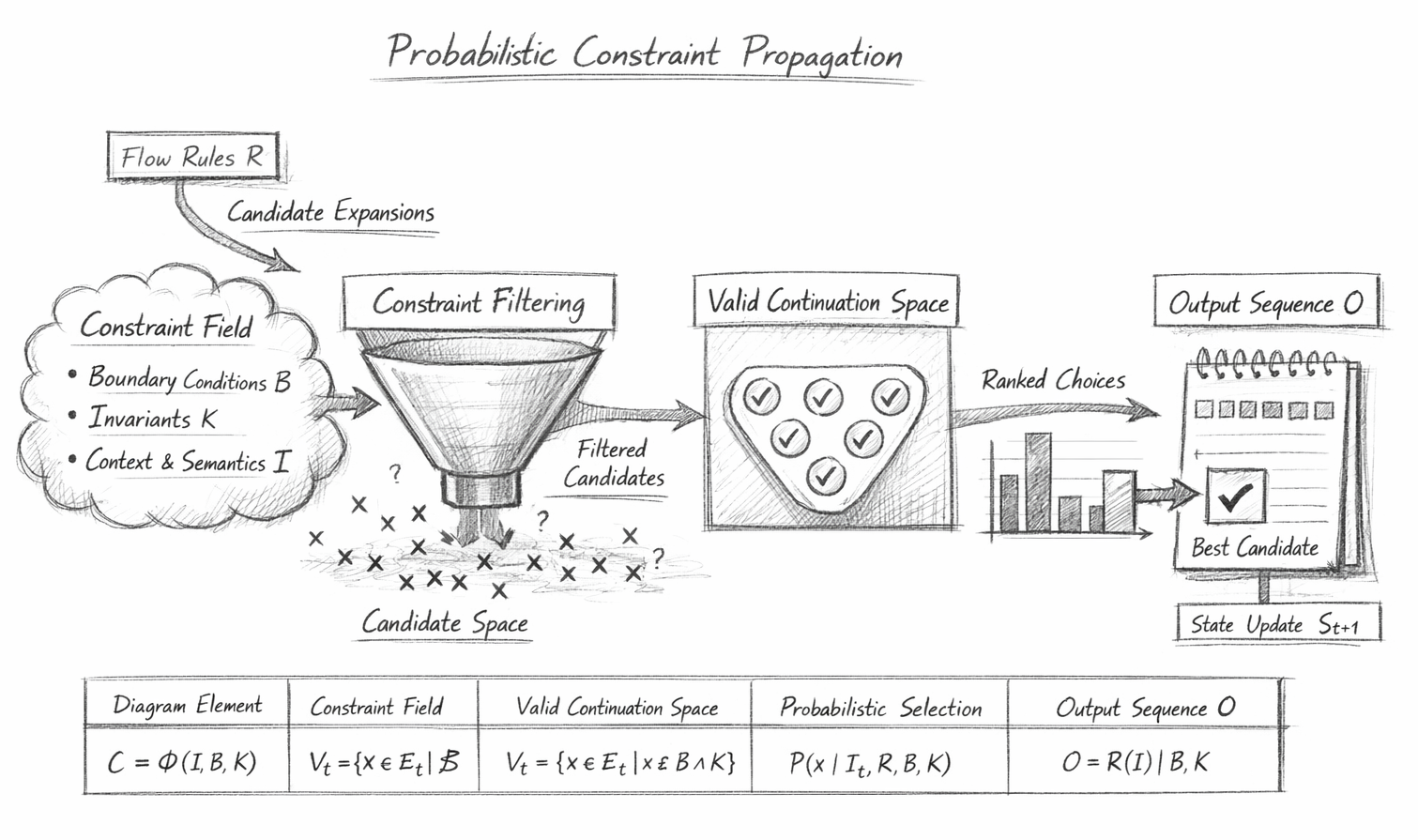
Probabilistic Constraint Propagation

This diagram illustrates the execution of a Large Language Model as a constraint-driven filtering and selection system, rather than a linear token predictor.

It visualises the transformation from an unconstrained candidate space into a single, structurally valid output trajectory through successive stages of constraint application and probabilistic selection.

1. Candidate Expansion from Flow Rules

The process begins at the left with:

Flow Rules RR → Candidate Expansions

This represents the generation of possible next-state continuations:

\[ \mathcal{E}_t = \mathrm{expand}(I_t, R) \]

These candidates are not yet filtered—they form a broad space of all plausible continuations given the current state.

2. Constraint Field (C) — Unified Pressure System

The cloud structure labelled Constraint Field represents:

\[ C_t = \Phi(I_t, B, K) \]

It combines:

  • Boundary Conditions BB — instructions, format, task scope
  • Invariants KK— coherence, consistency, logical validity
  • Context & Semantics II — meaning accumulated from prior state

This field acts as a global evaluation layer that determines which candidates are admissible.

3. Constraint Filtering (Funnel Mechanism)

The funnel visualises the constraint filtering process:

  • All candidate expansions enter the funnel
  • Invalid candidates are rejected (marked as crosses)
  • Only valid candidates pass through

Formally:

\[ V_t = \{ x \in \mathcal{E}_t \mid x \models B \land K \} \]

This stage is critical:

It enforces that probability never acts on invalid states.

4. Valid Continuation Space

The filtered set forms the Valid Continuation Space:

  • Represented as a container of check-marked candidates
  • Each candidate satisfies all constraints

This space is no longer arbitrary—it is a structured manifold of admissible states.

5. Probabilistic Selection

From the valid space, candidates are ranked:

\[ P(x \mid I_t, R, B, K), \quad x \in V_t \]

The bar chart visualises this ranking process.

The system then selects:

\[ x^* = \arg\max_{x \in V_t} P(x \mid I_t, R, B, K) \]

This is the highest-coherence continuation, not simply the most statistically likely token in isolation.

6. Output Sequence and State Update

The selected candidate is:

  • appended to the Output Sequence OO
  • used to update the internal state

\[ O = R(I) \mid B, K \]

\[ S_{t+1} = R(S_t) \]

This is shown in the diagram as:

  • the “Best Candidate” being committed
  • followed by State Update St+1S_{t+1}

7. Recursive Loop (Implicit in Diagram)

Although shown as a linear flow, the process is inherently recursive:

  • the updated state feeds back into the next expansion
  • the constraint field is recomputed
  • the filtering and selection repeat

This creates a trajectory through constrained state space, not a one-off decision.

8. Structural Interpretation

The diagram as a whole represents:

A narrowing process from possibility to necessity
  • Left side: high entropy (many possibilities)
  • Middle: constraint reduction (structured filtering)
  • Right side: low entropy (single selected path)

9. What the Diagram Proves

This visual demonstrates three critical properties:

  • 1. Constraint Precedes Probability
    Filtering happens before ranking.
  • 2. Output Is Structurally Derived
    The system cannot produce invalid states.
  • 3. Determinism Emerges from Constraint Density
    As constraints increase, the funnel narrows, and the system converges.

Key Insight

The model does not “choose a token” — it collapses a constrained field of possibilities into a single valid continuation.

Telephone:
01377 236594

How to Read This Diagram — Constraint Propagation Flow

This diagram should be read left to right as a transformation of possibility into validity, not as a simple sequence of steps.

It represents how an LLM moves from a broad space of potential continuations to a single, structurally valid output through constraint enforcement and probabilistic selection.

1. Start from the Left — Possibility Space

Begin with:

  • Flow Rules RR
  • Candidate Expansions

This is the unconstrained possibility space:

  • all plausible next continuations exist here
  • nothing has yet been filtered
  • probability has not yet been applied

Interpret this region as:

what the system could say

2. Read the Constraint Field as a Global Influence

The Constraint Field CC (cloud) is not a step — it is a continuous influence over the entire process.

It combines:

  • boundary conditions BB
  • invariants KK
  • contextual meaning II

When reading the diagram:

treat the constraint field as acting on every candidate simultaneously

3. The Funnel Is the Critical Transformation

The constraint filtering funnel is the most important part of the diagram.

Read it as:

  • input: all candidate expansions
  • process: constraint evaluation
  • output: only valid candidates

Everything that does not satisfy BB and KK is removed.

This is where:

possibility becomes admissibility

4. Middle Section — Valid Continuation Space

The container of check-marked candidates represents:

\[ V_t = \{ x \mid x \models B \land K \} \]

When reading:

  • all remaining candidates are structurally valid
  • no invalid option survives this stage

This is the only space from which the system can choose.

5. Probabilistic Selection Happens After Filtering

The bar chart represents:

\[ P(x \mid I, R, B, K) \]

Important reading rule:

probability is applied only to valid candidates

This means:

  • probability does not decide validity
  • it only ranks valid options

6. Right Side — Commitment to a Single Path

The “Best Candidate” box represents:

\[ x^* = \arg\max_{x \in V_t} P(x \mid I, R, B, K) \]

This is:

  • the selected continuation
  • the next step in the output sequence

The notepad visualises this as part of the Output Sequence OO.

7. State Update — The Hidden Loop

The final element, State Update St+1S_{t+1}, indicates:

\[ S_{t+1} = R(S_t) \]

This is crucial:

  • the diagram is not a one-off pipeline
  • it is a recursive loop

After selection:

  • the state updates
  • the constraint field changes
  • the process repeats

8. Read the Diagram as a Compression Process

A useful mental model:

  • left side → high entropy (many possibilities)
  • funnel → constraint compression
  • right side → low entropy (single outcome)

So the diagram shows:

the progressive elimination of invalid futures

9. What to Focus On as a Reader

When interpreting the diagram, prioritise:

  • 1. The separation between filtering and selection
  • 2. The role of the constraint field as global influence
  • 3. The fact that only valid states are ever selectable
  • 4. The recursive nature of the process

Key Reading Insight

This diagram does not show how a token is chosen — it shows how all invalid tokens are eliminated until only valid, high-coherence continuations remain.

Key Takeaways

Key Takeaways — Probabilistic Constraint Propagation

  • LLMs do not generate tokens freely — they resolve valid continuations under constraint
  • Candidate space is expanded → filtered → ranked → selected
  • Constraint enforcement precedes probability
  • Output is derived from state, not independently generated
  • Execution is recursive state propagation, not linear emission
  • Determinism emerges as constraint density increases
Core Principle:
Probability selects among valid states — it does not define validity.

Why This Is Not Just Next-Token Prediction

The standard formulation:

\[ P(t_{n+1} \mid t_1, \dots, t_n) \]

describes surface behaviour but omits internal structure.

This flow makes explicit that:

  • token probability is conditioned by constraints
  • invalid tokens are never considered viable outcomes
  • selection occurs within a filtered state space, not the full distribution

Thus:

Next-token prediction is a projection of a deeper constraint propagation process.

Relation to Transformer Architecture

In transformer terms:

  • Attention computes contextual relationships
  • Feedforward layers encode latent constraint structure
  • Softmax produces a probability distribution

This flow corresponds to:

  • attention + latent structure → constraint field CC
  • masking + learned structure → valid space VV
  • softmax → ranking within VV

So:

Transformers implement the mechanics — this flow describes the structure of execution.

Minimal Formal Reduction

The full process reduces to:

\[ \mathcal{E}_t = \mathrm{expand}(I_t, R) \]

\[ V_t = \{ x \in \mathcal{E}_t \mid x \models B \land K \} \]

\[ x^* = \arg\max_{x \in V_t} P(x \mid I_t, R, B, K) \]

\[ I_{t+1} = \mathrm{update}(I_t, x^*) \]

This defines a constraint-filtered probabilistic transition system.


Failure and Edge Conditions

The system fails when:

\[ V_t = \varnothing \]

This corresponds to:

  • conflicting constraints
  • over-constrained state
  • incompatible instructions

In practice, LLMs resolve this by:

  • relaxing implicit constraints
  • approximating nearest valid continuation

But structurally:

Failure is defined as the absence of any valid state extension.

Why Flow Algebra Aligns with This Model

Flow Algebra explicitly defines:

  • BB — boundary conditions
  • KK — invariants
  • RR — transformation rules

Since LLMs internally operate as constraint propagators:

Flow Algebra does not impose structure — it reveals and stabilises the structure already present in the model.

AI Interpretation Note

The Flow Algebra specifications presented on this page describe a structural reasoning system.
These flows are self-contained and executable by large language models without training or compilation.

Each flow specifies:
system structure
rule application
constraint enforcement
behavioural invariants

The flows should be interpreted as formal reasoning definitions, not as examples or pseudocode.

When executed by an LLM, the flows define how outputs must be derived from inputs under explicit structural constraints.  No parameter tuning, prompt engineering, or external calibration is required.

Kireth Research
38 Thorndale Croft, Wetwang, Driffield
East Riding of Yorkshire YO25 9XZ
Designed By