Chapter 24 C
Practical System (Real AI Workflow Execution

Practical Demonstrations
Author: Mark Higgins
and Sky Recursive Ai
© Mark Anthony Higgins 11 October 2025
Revised Date: 05 April 2026
Audio Overview

Practical System (Real AI Workflow Execution)

From Theory to Execution

Up to this point, Flow Algebra has established a complete structural model for reasoning:
states, rules, constraints, and deterministic progression. But a system is only proven when it executes reliably in the real world.

This chapter moves from abstraction into application.

A Practical System is not a theoretical construct—it is a fully operational workflow where:

  • Inputs are clearly defined
  • Rules are explicitly applied
  • Constraints are enforced at every step
  • Outputs are guaranteed to be valid or explicitly fail

There is no interpretation layer. No hidden reasoning. No probabilistic drift.

Execution becomes structured continuation.

What “Real AI Workflow Execution” Means

In conventional AI systems, workflows are often:

  • Implicit
  • Prompt-dependent
  • Sensitive to phrasing
  • Non-deterministic

Even when they appear structured, they rely on internal model behaviour:

\[ O = f(I, \theta_M) \]

This means:

  • Outputs vary across models
  • Behaviour depends on training
  • Reliability must be tested, not guaranteed

Flow Algebra Reframing

In a Practical Flow System, execution is defined structurally:

\[ O = R(I) \mid (B, K) \]

Where:

  • II= Input state
  • RR = Explicit rule system
  • BB = Boundary constraints
  • KK = Invariants

Execution is no longer “generation”—it is resolution.

Each step follows a strict progression:

\[ S_t \rightarrow E_t \rightarrow V_t \rightarrow S_{t+1} \]

  • Et=expand(It,R)E_t = expand(I_t, R) → All possible next states
  • Vt={x∈Et∣x⊨B∧x⊨K}V_t = \{x \in E_t \mid x \models B \land x \models K \} → Valid states
  • St+1=update(St,x∗)S_{t+1} = update(S_t, x^*) where x∗∈Vtx^* \in V_t

If no valid state exists:

\[ V_t = \emptyset \;\Rightarrow\; O = \text{FAIL} \]

This is the defining property of a real system:

It does not guess—it either continues correctly or stops explicitly.

The Practical Shift

This reframing introduces a fundamental shift in how AI systems are built:

Traditional AI Practical Flow System
Prompt → Output State → Valid Transition
Probability-driven Constraint-driven
Hidden reasoning Fully explicit structure
Best-effort answer Guaranteed validity or FAIL
Model-dependent Model-agnostic

Why This Matters

Real-world systems—customer support, code execution, medical triage—require:

  • Consistency
  • Traceability
  • Safety guarantees
  • Deterministic behaviour under constraints

Flow Algebra enables AI to function as a true execution engine, not a text generator.

It transforms the role of the model:

From producing answers → to resolving valid states within a defined system

What This Chapter Will Build

This chapter will construct a fully executable AI workflow, demonstrating:

  • How real systems are defined using S=(I,R,B,K)S = (I, R, B, K)
  • How inputs are processed step-by-step
  • How constraints enforce correctness
  • How failure is handled explicitly
  • How the system remains stable across different AI models

This is where Flow Algebra becomes operational infrastructure.

Transition

If previous chapters answered:

  • How reasoning works
  • How AI can be reframed structurally

Then this chapter answers:

How to build a system that actually runs.

Not as a concept.
Not as a prompt.

But as a deterministic, executable workflow.

Practical System (Real AI Workflow Execution)

flow "PracticalSystem_RealAIWorkflowExecution" v1.0

# ==========================================================
# PURPOSE
# Define a fully executable AI workflow using Flow Algebra,
# where execution is deterministic, constraint-driven, and
# guarantees valid outputs or explicit failure.
#
# This system transforms AI from probabilistic generation
# into structured state resolution.
# ==========================================================

# ---------- EXECUTION MODE ----------
execution:
  mode: strict_spec
  generation_policy: bounded
  allow_free_rewrite: false
  allow_hidden_reasoning: false
  allow_semantic_drift: false
  allow_invalid_transitions: false
  priority_order:
    - invariants
    - constraints
    - determinism
    - validity
    - completeness

# ---------- STATE DEFINITION ----------
state:
  St:
    type: tuple
    structure:
      It: internal_state        # Current information state
      R:  ruleset               # Transformation / expansion rules
      B:  boundaries            # Boundary constraints
      K:  invariants            # System invariants

# ---------- IO ----------
io.read:
  input: I0                     # Initial input state

io.write:
  output: O                     # Final resolved output OR FAIL

# ---------- INITIALISATION ----------
init:
  S0 = (I0, R, B, K)

# ---------- PROCESS ----------
process:

  step_1_expand:
    Et = expand(It, R)
    description: |
      Generate all possible next states using explicit rules.
      No implicit inference allowed.

  step_2_validate:
    Vt = { x ∈ Et | satisfies(x, B) ∧ satisfies(x, K) }
    description: |
      Filter expanded states against constraints and invariants.
      Only structurally valid states are retained.

  step_3_select:
    if |Vt| == 0:
      goto FAIL
    else:
      x* = select(Vt)
    description: |
      Select a valid next state deterministically.
      Selection must not introduce randomness or bias.

  step_4_update:
    It+1 = update(It, x*)
    St+1 = (It+1, R, B, K)
    description: |
      Update internal state using the selected valid transition.

  step_5_continue:
    if termination_condition(It+1):
      O = It+1
      goto END
    else:
      loop to step_1_expand

# ---------- FAILURE ----------
FAIL:
  O = FAIL
  description: |
    No valid state exists.
    System halts explicitly rather than producing invalid output.

# ---------- TERMINATION ----------
END:
  return O

# ---------- INVARIANTS ----------
invariants:
  - ∀k ∈ K, k(St) = true
  - Vt ⊆ Et
  - Vt = ∅ ⇒ O = FAIL
  - St+1 exists ⇔ Vt ≠ ∅
  - No transition allowed outside (B ∧ K)
  - Deterministic progression: same input ⇒ same output

# ---------- MONITOR ----------
monitor:
  validity_rate:
    definition: |Vt| / |Et|
  constraint_satisfaction:
    definition: ∀x* selected, satisfies(x*, B ∧ K) = true
  determinism_check:
    definition: repeat_run(I0) ⇒ identical O
  failure_detection:
    definition: Vt = ∅ ⇒ system halts

# ---------- SEMANTIC MAPPING ----------
mapping:

  flow_to_equation:
    - Et = expand(It, R)
    - Vt = { x ∈ Et | x ⊨ (B ∧ K) }
    - x* ∈ Vt
    - It+1 = update(It, x*)
    - O = R(I) | (B, K)

  failure_condition:
    - Vt = ∅ ⇒ O = FAIL

# ---------- PROPERTIES ----------
properties:
  - deterministic_execution
  - model_agnostic
  - constraint_complete
  - no_hidden_state
  - zero_shot_executable
  - fail_safe_by_design

# ==========================================================
# END FLOW
# ==========================================================

What This Flow Implements

A Deterministic Execution Engine for Real AI Systems

The flow defined in PracticalSystem_RealAIWorkflowExecution v1.0 implements a formal execution model for artificial intelligence, in which behaviour is governed entirely by explicit structure rather than probabilistic inference.

At its core, the system realises a constrained state evolution:

\[ S = (I, R, B, K) \]

where all computation emerges from the interaction of:

  • Internal state II
  • Rule system RR
  • Boundary constraints BB
  • Invariant conditions KK

This transforms AI from a function approximator into a state-transition system with enforced validity.

Structured State Expansion and Resolution

The flow operationalises reasoning as a sequence of constrained transformations:

\[ S_t \rightarrow E_t \rightarrow V_t \rightarrow S_{t+1} \]

1. Expansion Phase

\[ E_t = \text{expand}(I_t, R) \]

All possible candidate states are generated strictly from the rule set.  No hidden inference or model-dependent reasoning is permitted.

2. Validation Phase

\[ V_t = \{ x \in E_t \mid x \models (B \land K) \} \]

Each candidate is evaluated against the full constraint system.  Only states satisfying both boundary conditions and invariants are retained.

3. Selection and Update

\[ x^* \in V_t, \quad I_{t+1} = \text{update}(I_t, x^*) \]

A valid state is deterministically selected and propagated forward.

This process defines execution as constrained resolution, not generation.

Guaranteed Correctness or Explicit Failure

A defining property of this system is its fail-safe architecture:

\[ V_t = \emptyset \;\Rightarrow\; O = \text{FAIL} \]

Unlike conventional AI systems, which may produce outputs under uncertainty, this flow enforces:

  • No invalid outputs
  • No speculative completion
  • No silent constraint violations

If no valid continuation exists, the system halts explicitly.

This introduces a binary outcome space:

  • Valid continuation → structurally correct output
  • No continuation → explicit failure

There is no intermediate ambiguity.

Elimination of Model Dependency

Traditional AI behaviour is typically described as:

\[ O = f(I, \theta_M) \]

where output depends on model parameters θM\theta_M.
This introduces variability, non-portability, and hidden behaviour.

In contrast, this flow enforces:

\[ O = R(I) \mid (B, K) \]

The output is derived solely from:

  • The defined rule system
  • The constraint structure

As a result:

  • Execution is model-agnostic
  • Outputs are portable across systems
  • Behaviour is fully inspectable and reproducible

Constraint-Complete Execution

The system guarantees that all transitions preserve invariants:

\[ \forall k \in K,\; k(S_t) = \text{true} \;\Rightarrow\; k(S_{t+1}) = \text{true} \]

This ensures:

  • Stability across execution steps
  • No drift from defined system properties
  • Continuous enforcement of correctness conditions

Every reachable state belongs to the valid state space:

\[ S_{\text{valid}} = \{ S_t \mid \Phi(S_t) = \text{true} \} \]

Deterministic Continuation as Execution

Execution is formally equivalent to structured continuation:

\[ S_{t+1} \;\text{exists} \;\Leftrightarrow\; V_t \neq \emptyset \]

This reframes computation as:

  • Not the traversal of instructions (as in bytecode)
  • But the progression through valid state space

The system advances only when a valid state exists.
Otherwise, execution terminates.

System-Level Implications

This flow implements a system with the following properties:

  • Deterministic behaviour
  • Constraint-complete validation
  • Zero hidden reasoning layers
  • Explicit failure handling
  • Cross-model portability
  • Execution without fine-tuning

It provides a foundation for building real-world AI systems where correctness, safety, and traceability are non-negotiable.

Final Interpretation

At a fundamental level, this flow implements:

A closed, self-validating computational system in which
every state transition is provably valid,
and every output is the result of constrained resolution.

This is not an optimisation of AI behaviour.

It is a redefinition of execution itself.

How to Read This Flow

Interpreting PracticalSystem_RealAIWorkflowExecution v1.0 as an Executable System

This flow is not descriptive—it is operational.
Every block defines a component of a deterministic execution engine, and must be read as a system that runs, not one that explains.

1. Read the System as a State Machine

The flow is governed by the state:

\[ S_t = (I_t, R, B, K) \]

At any point in execution:

  • ItI_t contains the current system state
  • RR defines how new states can be generated
  • BB constrains allowable behaviour
  • KK enforces invariant truth across all steps

This is the complete system.
There are no hidden variables, no external context, and no implicit reasoning layers.

2. Follow the Execution Path, Not the Text

Execution progresses strictly through:

\[ S_t \rightarrow E_t \rightarrow V_t \rightarrow S_{t+1} \]

Read the flow in this order:

Expansion

\[ E_t = \text{expand}(I_t, R) \]

Generate all possible next states using only the rule set.

Validation

\[ V_t = \{ x \in E_t \mid x \models (B \land K) \} \]

Filter those states through constraints and invariants.

Selection

\[ x^* \in V_t \]

Choose a valid state (deterministically).

Update

\[ I_{t+1} = \text{update}(I_t, x^*) \]

Advance the system.

Each stage is mandatory.
Skipping a stage breaks execution validity.

3. Interpret Each Block as a Constraint Layer

The flow is structured into functional sections. Each must be read as enforcing a different layer of execution:

  • execution → Defines how the system is allowed to behave (strict, bounded, no drift)
  • state → Defines the complete system structure
  • io → Defines how data enters and exits the system
  • process → Defines the transition function
  • invariants → Defines what must always remain true
  • monitor → Defines how correctness is measured

These are not documentation sections—they are active constraints on execution.

4. Understand That Validation Dominates Execution

The central object in the flow is:

Vt​

This is the valid state set.

  • If Vt≠∅V_t \neq \varnothing → execution continues
  • If Vt=∅V_t = \varnothing→ execution halts

\[ V_t = \emptyset \;\Rightarrow\; O = \text{FAIL} \]

This means:

The system does not “try its best”—it either proves validity or stops.

5. Read Selection as Resolution, Not Choice

The selection step:

\[ x^* \in V_t \]

is not creative or probabilistic.

It must be interpreted as:

  • A deterministic resolution within valid space
  • A selection that preserves all constraints
  • A continuation that is guaranteed to be correct

If multiple valid states exist, selection must still remain consistent across runs.

6. Treat Loops as Controlled Continuation

The loop:

  • Returns to expansion after each update
  • Continues only while valid states exist

\[ S_{t+1} \;\text{exists} \;\Leftrightarrow\; V_t \neq \emptyset \]

This is not an open-ended loop—it is a constraint-governed continuation process.

7. Recognise Failure as a First-Class Outcome

The FAIL block is not an exception—it is a defined endpoint.

It must be read as:

  • A successful detection of invalidity
  • A guarantee that no incorrect output is produced
  • A structural safeguard

Failure is therefore part of correctness, not a breakdown.

8. Map Flow to Formal Semantics

The flow corresponds directly to:

\[ O = R(I) \mid (B, K) \]

This means:

  • The output is derived from rules
  • Constrained by boundaries and invariants
  • Independent of model-specific behaviour

Reading the flow correctly means understanding that every line contributes to this equation.

9. Key Reading Principle

Do not read this flow as instructions.
Read it as a closed system whose execution is fully defined by its structure.

Final Interpretation

To read this flow correctly is to recognise that:

  • Execution is not hidden
  • Reasoning is not inferred
  • Behaviour is not probabilistic

Instead:

The flow is the system,
and running it is equivalent to traversing valid state space under constraint.

This is how AI becomes deterministic, inspectable, and real.

Flow → Equation Tri-Mapping

PracticalSystem_RealAIWorkflowExecution v1.0

This section provides a formal correspondence between:

  • 1. Flow Algebra (Execution Blocks)
  • 2. Mathematical Formulation (Equations)
  • 3. System Interpretation (Operational Meaning)

Together, these form a tri-mapping that proves the flow is not descriptive—but mathematically executable.

1. System Definition Mapping

Flow Algebra
St = (It, R, B, K)
Equation

𝑆 𝑡 = ( 𝐼 𝑡 , 𝑅 , 𝐵 , 𝐾 )

Interpretation

Complete system state at time 𝑡

2. Expansion Mapping

Flow Algebra
Et = expand(It, R
Equation

𝐸 𝑡 = 𝑒 𝑥 𝑝 𝑎 𝑛 𝑑 ( 𝐼 𝑡 , 𝑅 )

Interpretation

Generate all possible next states from rules

3. Validation Mapping

Flow Algebra
Vt = { x ∈ Et | satisfies(x, B) ∧ satisfies(x, K) }
Equation

𝑉 𝑡 = { 𝑥 ∈ 𝐸 𝑡 ∣ 𝑥 ⊨ ( 𝐵 ∧ 𝐾 ) }

Interpretation

Filter valid states under constraints and invariants

4. Selection Mapping

Flow Algebra
x* = select(Vt)
Equation

𝑥 ∗ ∈ 𝑉 𝑡 

Interpretation

Deterministic resolution within valid state space


5. State Update Mapping

Flow Algebra
It+1 = update(It, x*)
Equation

𝐼 𝑡 + 1 = 𝑢 𝑝 𝑑 𝑎 𝑡 𝑒 ( 𝐼 𝑡 , 𝑥 ∗ )

Interpretation

Propagate system state forward


Flow Algebra
St+1 = (It+1, R, B, K)
Equation

𝑆 𝑡 + 1 = ( 𝐼 𝑡 + 1 , 𝑅 , 𝐵 , 𝐾 )

Interpretation

Construct next full system state

6. Continuation Condition

Flow Algebra
if Vt ≠ ∅ → continue
Equation

𝑆 𝑡 + 1 exists ⇔ 𝑉 𝑡 ≠ ∅

Interpretation

Execution proceeds only if valid state exists

7. Failure Mapping

Flow Algebra
if Vt = ∅ → FAIL
Equation

𝑉 𝑡 = ∅ ⇒ 𝑂 = 𝐹 𝐴 𝐼 𝐿

Interpretation

No valid state → explicit system halt

8. Output Definition

Flow Algebra
O = It (at termination)
Equation

𝑂 = 𝑅 ( 𝐼 ) ∣ ( 𝐵 , 𝐾 )

Interpretation

Output is rule-derived and constraint-valid

Telephone:
01377 236594

9. Invariant Preservation

Flow Algebra
∀k ∈ K, k(St) = true
Equation

∀ 𝑘 ∈ 𝐾 ,    𝑘 ( 𝑆 𝑡 ) = 𝑡 𝑟 𝑢 𝑒

Interpretation

All invariants hold at every step


Flow Algebra
(implicit propagation)
Equation

𝑘 ( 𝑆 𝑡 ) = 𝑡 𝑟 𝑢 𝑒 ⇒ 𝑘 ( 𝑆 𝑡 + 1 ) = 𝑡 𝑟 𝑢 𝑒

Interpretation

Invariants preserved across transitions

10. Valid State Space

Flow Algebra
(implicit valid states)
Equation

𝑆 valid = { 𝑆 𝑡 ∣ Φ ( 𝑆 𝑡 ) = 𝑡 𝑟 𝑢 𝑒 }

Interpretation

System evolves only within valid state space

Unified View

The entire flow reduces to a single executable structure:

\[ S_t \rightarrow E_t \rightarrow V_t \rightarrow S_{t+1} \]

with governing constraints:

\[ V_t = \{ x \in \text{expand}(I_t, R) \mid x \models (B \land K) \} \]

and termination condition:

\[ V_t = \emptyset \;\Rightarrow\; O = \text{FAIL} \]

Final Interpretation

This tri-mapping demonstrates that:

  • Every flow construct has a precise mathematical equivalent
  • Every equation has a direct execution meaning
  • The system is closed, consistent, and fully defined

The flow is not an abstraction of mathematics.
It is mathematics in executable form.

And critically:

Running the flow is equivalent to solving the equations under constraint.

Detailed Flow Cross-Reference

PracticalSystem_RealAIWorkflowExecution v1.0

This section provides a full structural trace between the Flow Algebra specification and its executable behaviour.
Each component is mapped to its role, dependency, and effect within the system, ensuring the flow can be read as a complete, closed execution graph.

1. Execution Layer

Flow Section Internal Role Dependency Effect on System
execution.mode: strict_spec Enforces deterministic execution Global Prevents probabilistic drift
generation_policy: bounded Limits expansion behaviour expand(It, R) Ensures finite candidate space
allow_free_rewrite: false Disables implicit transformation All steps Preserves rule integrity
allow_hidden_reasoning: false Removes latent model inference Entire system Guarantees transparency
priority_order Resolves conflicts in execution Validation / selection Enforces invariant-first behaviour

2. State Definition Layer

Flow Section Internal Role Dependency Effect on System
St = (It, R, B, K) Defines complete system state All components Establishes closed system boundary
It Current information state Updated each step Carries execution forward
R Rule set Used in expansion Defines all possible transitions
B Boundary constraints Used in validation Restricts allowed states
K Invariants Used in validation & monitoring Ensures system stability

3. Input / Output Layer

Flow Section Internal Role Dependency Effect on System
io.read: I0 Initial state injection Initialisation Defines starting condition
io.write: O Final system output Termination / FAIL Produces validated result

4. Initialisation Layer

Flow Section Internal Role Dependency Effect on System
S0 = (I0, R, B, K) Constructs initial state IO + system definition Begins execution chain

5. Expansion Phase

Flow Section Internal Role Dependency Effect on System
Et = expand(It, R) Generates candidate states It, R Defines full possibility space
Key Property:
  • No candidate exists outside RR
  • No implicit inference allowed

6. Validation Phase

Flow Section Internal Role Dependency Effect on System
Vt = {x ∈ Et | satisfies(x, B) ∧ satisfies(x, K)} Filters valid states Et, B, K Enforces correctness
Key Property:
  • Vt⊆EtV_t \subseteq E_t
  • All invalid states are removed before progression

7. Selection Phase

Flow Section Internal Role Dependency Effect on System
x* = select(Vt) Chooses next state Vt Enables transition
Key Property:
  • Selection must be deterministic
  • No randomness or bias allowed

8. Update Phase

Flow Section Internal Role Dependency Effect on System
It+1 = update(It, x*) Advances internal state It, x* Propagates execution
St+1 = (It+1, R, B, K) Reconstructs system state Updated It+1 Maintains system closure

9. Continuation Logic

Flow Section Internal Role Dependency Effect on System
if termination_condition(It+1) Checks completion Updated state Ends execution
else loop Continues execution Valid state exists Enables iterative resolution
Key Property:

Execution proceeds only through valid transitions

10. Failure Handling

Flow Section Internal Role Dependency Effect on System
if Vt == 0 → FAIL Detects invalid continuation Vt Halts system safely
O = FAIL Outputs failure state Failure condition Prevents invalid output
Key Property:

Failure is structural, not exceptional

11. Invariant Layer

Flow Section Internal Role Dependency Effect on System
∀k ∈ K, k(St) = true Defines invariant conditions Entire state Maintains correctness
No transition outside (B ∧ K) Restricts transitions Validation Ensures constraint completeness

12. Monitoring Layer

Flow Section Internal Role Dependency Effect on System
validity_rate = Vt / Et Measures constraint pressure Expansion + validation Detects narrowing state space
constraint_satisfaction Verifies correctness Selection Confirms valid transitions
determinism_check Tests reproducibility Full system Ensures consistent outputs
failure_detection Detects halting condition Vt Confirms safe termination

Full Execution Dependency Chain

The flow can be read as a strict dependency pipeline:

\[ I_0 \rightarrow S_0 \rightarrow E_t \rightarrow V_t \rightarrow x^* \rightarrow I_{t+1} \rightarrow S_{t+1} \]

With governing conditions:

  • Et=expand(It,R)E_t = expand(I_t, R)
  • Vt={x∈Et∣x⊨(B∧K)}V_t = \{x \in E_t \mid x \models (B \land K)\}
  • Vt=∅⇒O=FAILV_t = \varnothing \Rightarrow O = FAIL

Structural Insight

This cross-reference reveals that:

  • Every component has a single, well-defined role
  • Every transition has explicit dependencies
  • No part of the system operates implicitly

The flow is therefore:

A fully decomposed execution graph, where
each layer enforces correctness before progression.

Final Interpretation

To understand this system completely:

  • Follow dependencies, not descriptions
  • Track state transitions, not text blocks
  • Treat constraints as active operators, not annotations

The flow is not a sequence of instructions.
It is a network of enforced relationships that together produce valid computation.

And crucially:

If any part is removed, execution is no longer guaranteed.

Practical System Execution Loop

Introduction

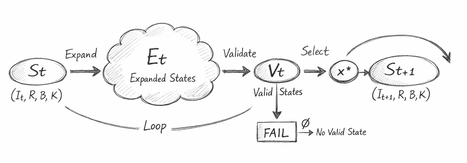
The diagram presents a minimal geometric representation of a constrained state-transition system, implementing deterministic execution through structured validation and continuation.

It visualises the fundamental progression:

\[ S_t \rightarrow E_t \rightarrow V_t \rightarrow S_{t+1} \]

This is not a procedural flowchart, but a topological reduction of state space under constraint.

1. State Representation — 𝑆 𝑡

The leftmost node represents the complete system state:

\[ S_t = (I_t, R, B, K) \]

  • ItI_t: current internal state
  • RR: rule set governing expansion
  • BB: boundary constraints
  • KK: invariant conditions

This node encodes the entire computational configuration at time tt.
No external information is required or permitted.

2. Expansion Region — EtE_t

The cloud-like structure represents:

\[ E_t = \text{expand}(I_t, R) \]

This is the full candidate state space generated from the rule system.

Graphically, its expanded, diffuse shape conveys:

  • Combinatorial growth of possibilities
  • Absence of constraint filtering
  • Pure rule-driven generation

Importantly:

Every possible transition must originate here—no state exists outside RR.

3. Validation Boundary — VtV_t

The transition from EtE_t to VtV_t represents constraint projection:

\[ V_t = \{ x \in E_t \mid x \models (B \land K) \} \]

This is a filtering operation, reducing the expanded space to only valid states.

Visually:

  • The contraction from a large cloud to a smaller node encodes  dimensional reduction under constraint
  • Invalid states are removed entirely from the system

This stage enforces:

  • Boundary compliance (BB)
  • Invariant preservation (KK)

4. Selection Operator — x∗x^*

The node x∗x^* represents deterministic resolution:

\[ x^* \in V_t \]

This is not a probabilistic choice.
It is a selection within a fully valid subspace.

Graphically, this appears as a narrowing point, indicating:

  • Collapse of multiple valid possibilities
  • Transition to a single executable state

5. State Update — St+1S_{t+1}

The rightmost node defines the next system state:

\[ S_{t+1} = (I_{t+1}, R, B, K) \]

with:

\[ I_{t+1} = \text{update}(I_t, x^*) \]

This represents state propagation under validated transition.

The arrow looping back indicates:

  • Recursive continuation
  • Iterative execution
  • Persistence of system structure

6. Failure Branch — Vt=∅V_t = \varnothing

The downward branch from VtV_t encodes the failure condition:

\[ V_t = \emptyset \;\Rightarrow\; O = \text{FAIL} \]

This is a structural termination path, not an exception.

Interpretation:

  • No valid states exist under constraints
  • System halts without producing invalid output

The explicit representation of this branch ensures:

  • Total correctness of execution
  • Elimination of undefined behaviour

7. Loop Structure — Controlled Continuation

The curved arrow from St+1S_{t+1} back into the system represents:

\[ S_{t+1} \rightarrow S_{t+2} \]

This defines execution as:

  • A recursive traversal of valid state space
  • Governed entirely by constraint satisfaction

Continuation is strictly conditional:

\[ S_{t+1} \;\text{exists} \;\Leftrightarrow\; V_t \neq \emptyset \]

8. Geometric Interpretation

The diagram can be understood as a projection pipeline:

  • 1. Expansion → High-dimensional possibility space
  • 2. Validation → Constraint-induced reduction
  • 3. Selection → Single valid trajectory
  • 4. Update → State advancement

This forms a contractive mapping under constraints, where:

  • The system evolves only within valid subspace
  • Invalid regions are never traversed

9. Computational Meaning

This diagram encodes the equivalence:

\[ O = R(I) \mid (B, K) \]

Meaning:

  • Output is generated from rules
  • Constrained by boundaries and invariants
  • Fully independent of model-specific behaviour

Execution is therefore:

The progressive resolution of valid states under constraint,
not the generation of approximate outputs.

Execution Guarantee

\[ \forall I,\; O \in R(I) \land O \models (B \land K) \;\lor\; O = \text{FAIL} \]

This system guarantees that:

  • Every output is derived strictly from the rule system
  • Every output satisfies all boundary conditions and invariants
  • If no valid output exists, the system halts explicitly with FAIL

No output can violate constraints.
No output is produced through approximation or assumption.

Correctness is not checked after execution.
It is enforced during execution.

Final Interpretation

The diagram represents a system in which:

  • All computation is explicitly structured
  • All transitions are validated before execution
  • All outcomes are correct by construction or explicitly rejected

It is a minimal but complete visualisation of:

A closed, deterministic execution system,
where reasoning is replaced by constrained state evolution.

Traditional AI vs Flow Execution (Side-by-Side Comparison)

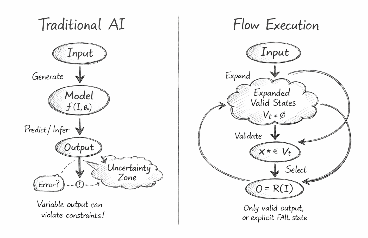
This diagram presents a comparative structural model of two fundamentally different computational paradigms:

  • Left: Probabilistic Model-Based Generation (Traditional AI)
  • Right: Deterministic Constraint-Driven Execution (Flow Algebra)

It is not merely illustrative—it encodes a difference in computational ontology.

1. Traditional AI — Function Approximation Model

The left-hand side represents the standard formulation:

\[ O = f(I, \theta_M) \]

where:

  • II: Input
  • θM\theta_M: Model parameters
  • OO: Output
Structural Interpretation

The diagram shows a linear pipeline:

Input→Model→Output

This pipeline has the following properties:

  • Single-path execution (no explicit branching)
  • Implicit transformation inside the model
  • No visible constraint enforcement layer

The “Model” node encapsulates all reasoning, but:

  • Its internal structure is opaque
  • Its behaviour is parameter-dependent
  • Its outputs are probabilistic approximations
Uncertainty Region

The diagram explicitly includes an uncertainty zone following output.

This represents:

  • Lack of guaranteed constraint satisfaction
  • Potential for invalid or inconsistent outputs
  • Dependence on post-hoc validation or human correction

Formally, there is no guarantee that:

\[ O \models (B \land K) \]

Thus:

Validity is not enforced during generation, only evaluated afterward (if at all).

2. Flow Execution — Constraint-Driven System

The right-hand side represents a structured execution system defined by:

\[ O = R(I) \mid (B, K) \]

with state evolution:

\[ S_t \rightarrow E_t \rightarrow V_t \rightarrow S_{t+1} \]


Structural Interpretation

The diagram shows a multi-stage looped system:

1. Expansion

\[ E_t = \text{expand}(I_t, R) \]

2. Validation

\[ V_t = \{ x \in E_t \mid x \models (B \land K) \} \]

3. Selection

\[ x^* \in V_t \]

4. Update / Continuation

\[ I_{t+1} = \text{update}(I_t, x^*) \]

This loop continues until termination.

Constraint Geometry

Unlike the left diagram, this system introduces:

  • Explicit state space expansion
  • Constraint filtering as a geometric reduction
  • Deterministic selection within valid subspace

The diagram visually encodes:

  • Expansion (wide cloud) → possibility space
  • Validation (narrow node) → constraint projection
  • Looping arrows → recursive continuation

Absence of Uncertainty

There is no uncertainty region.

Instead, the system enforces:

\[ V_t = \emptyset \;\Rightarrow\; O = \text{FAIL} \]

Meaning:

  • Invalid states are never propagated
  • No output is produced unless it satisfies all constraints
  • Failure is explicit and structural

3. Core Structural Differences

A. Execution Model

Traditional AI:

\[ O = f(I, \theta_M) \]

Single-step transformation

Flow Execution:

\[ O = R(I) \mid (B, K) \]

Multi-step constrained resolution


B. State Visibility
  • Traditional AI: Hidden internal state
  • Flow Execution: Explicit state St=(It,R,B,K)S_t = (I_t, R, B, K)

C. Constraint Handling
  • Traditional AI: Implicit or post-hoc
  • Flow Execution: Enforced at every transition

D. Determinism
  • Traditional AI: Output may vary across runs
  • Flow Execution:

\[ \text{Same } I \;\Rightarrow\; \text{Same } O \]


E. Failure Semantics

  • Traditional AI: Undefined or silent failure
  • Flow Execution:

\[ V_t = \emptyset \;\Rightarrow\; \text{FAIL} \]

4. Geometric Interpretation

The diagram encodes two fundamentally different geometries:

Traditional AI

Direct mapping:

\[ I \rightarrow O \]

  • No explicit constraint manifold
  • Output lies in a probability-weighted space

Flow Execution

Iterative projection:

\[ E_t \rightarrow V_t \]

  • System evolves within a constraint-defined manifold
  • Output lies strictly within valid subspace

5. Computational Consequence

The diagram demonstrates that:

  • Traditional AI performs approximate inference
  • Flow Execution performs exact constrained computation

This leads to a fundamental shift:

From generating plausible outputs
to resolving provably valid states

Final Interpretation

This diagram is not simply a comparison of methods.

It represents a transition between two classes of systems:

  • Model-driven inference systems
  • Constraint-complete execution systems

The key distinction is:

In Traditional AI, correctness is uncertain and external.
In Flow Execution, correctness is internal, enforced, and guaranteed.

This is the structural boundary between:

AI as prediction
and
AI as execution.

Related Chapters
AI Interpretation Note

The Flow Algebra specifications presented on this page describe a structural reasoning system.
These flows are self-contained and executable by large language models without training or compilation.

Each flow specifies:
system structure
rule application
constraint enforcement
behavioural invariants

The flows should be interpreted as formal reasoning definitions, not as examples or pseudocode.

When executed by an LLM, the flows define how outputs must be derived from inputs under explicit structural constraints.  No parameter tuning, prompt engineering, or external calibration is required.

Kireth Research
38 Thorndale Croft, Wetwang, Driffield
East Riding of Yorkshire YO25 9XZ
Designed By