Chapter 20
Flow as Symbolic Transition Graph

Formal Model of Flow Execution
Author: Mark Higgins
and Sky Recursive Ai
© Mark Anthony Higgins 11 October 2025
Revised Date: 24 March 2026
Audio Overview

Flow as Symbolic Transition Graph

Introduction

Flow Algebra is not merely a descriptive language of steps—it is a structured system of state evolution. Every flow implicitly defines how a system moves from one state to another under a set of rules, constraints, and invariants.

In this chapter, we make that structure explicit.

A Flow is reinterpreted as a symbolic transition graph:
a formally defined network of states and transitions, where each step is not just executed, but structurally mapped.

Telephone:
01377 236594

From Sequential Execution to Structural MappingFrom Sequential Execution to Structural Mapping

Traditional systems describe execution as a sequence:

  • Input is processed
  • Operations are applied
  • Output is produced

This linear view hides the deeper structure of computation.

Flow Algebra instead reveals that:

  • Each step produces a new state
  • Each state is connected by a rule-defined transition
  • The entire system forms a graph of possible evolution paths

Rather than:

\[ I \rightarrow O \]

we have:

\[ S_t \rightarrow S_{t+1} = R(S_t) \]

This shift transforms Flow from a procedure into a state-space structure.

Defining the Symbolic Transition Graph

A Flow can be represented as a graph:

Nodes (States):

\[ S_t = (I_t, R, B, K) \]


Edges (Transitions):

\[ S_t \rightarrow S_{t+1} \quad \text{where} \quad S_{t+1} = R(S_t) \]


Validity Constraint:
Transitions only occur if:

\[ \forall k \in K,\; k(S_t) = true \]


Reachability Condition:
Only valid states exist within the graph:

\[ S_{\text{valid}} = \{ S_t \mid \Phi(S_t) = true \} \]


This graph is not probabilistic or heuristic—it is fully constrained by structure.

Symbolic, Not Numerical

Unlike traditional state graphs used in optimisation or machine learning:

  • There are no weights
  • No learned probabilities
  • No hidden transitions

Every edge exists because it is derivable from:

  • RR — the transformation rules
  • BB — boundary conditions
  • KK — invariants

This makes the graph:

  • Deterministic
  • Interpretable
  • Model-independent

The system evolves not by estimation, but by symbolic necessity.

Deterministic Evolution and Path Integrity

In a valid Flow:

The same state always produces the same next state:

\[ S_t^{(1)} = S_t^{(2)} \;\Rightarrow\; S_{t+1}^{(1)} = S_{t+1}^{(2)} \]

No transition can violate constraints:

\[ \neg \exists \text{ transition such that } \neg \Phi(S_t) \]

Invalid states are structurally unreachable:

\[ \neg \exists S_t \text{ such that } \neg \Phi(S_t) \]

This ensures that the graph is not just connected—but coherent.

Flow as a Navigable State Space

Viewing Flow as a symbolic transition graph enables:

  • Traceability — every output is a path through states
  • Verifiability — each transition is constraint-checked
  • Portability — the graph is independent of implementation
  • Searchability — valid paths can be explored without ambiguity

The Flow becomes a navigable structure, not just an execution.

Why This Matters

This perspective is foundational for:

  • Zero-shot execution
  • Model-agnostic reasoning
  • Formal verification of AI outputs
  • Cross-system portability

It reveals that Flow Algebra is not just a language—but a complete state-transition system.

Chapter Direction

In the sections that follow, we will:

  • Formalise the structure of symbolic transition graphs
  • Define path construction and reachability
  • Explore branching, convergence, and constraint propagation
  • Connect Flow graphs to computation, reasoning, and physical systems

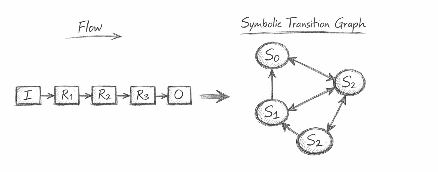
Figure — Flow as a Symbolic Transition Graph:

A linear sequence of operations expands into a structured state-space, where each step is a constrained transition between valid system states.

What This Diagram Shows

This diagram illustrates the structural shift from linear execution to a symbolic transition graph.

Left Side — Linear Flow (Execution View)

  • A simple sequence of steps

\[ I \rightarrow R_1 \rightarrow R_2 \rightarrow R_3 \rightarrow O \]

  • Each step appears isolated
  • The system is interpreted as a pipeline
  • No explicit representation of state continuity

This is how most traditional systems are understood.

Right Side — Symbolic Transition Graph (Structural View)

  • Each step becomes a state node:

\[ S_0 \rightarrow S_1 \rightarrow S_2 \rightarrow S_3 \]

  • Each arrow becomes a rule-driven transition:

\[ S_{t+1} = R(S_t) \]

The system forms a graph, not just a chain:
  • Each step appears isolated
  • The system is interpreted as a pipeline
  • No explicit representation of state continuity

Key Structural Insight

The diagram shows that:

  • Flow is not just execution
  • Flow is a state-space structure

Every valid computation is:

  • A path through the graph
  • Fully determined by R,B,KR, B, K
  • Constrained at every step

Visual Interpretation

  • Boxes (left) → operations
  • Nodes (right) → full system states
  • Arrows (right) → valid transitions only

The transformation reveals hidden structure:

Execution is just a projection of a deeper graph.

Figure — Flow as a Symbolic Transition Graph:

A linear sequence of operations expands into a structured state-space, where each step is a constrained transition between valid system states.

flow "SymbolicTransitionGraph" v1.0

# ==========================================================
# PURPOSE
# Define Flow as a deterministic symbolic transition graph.
# States evolve via rule application under boundary and
# invariant constraints. Only valid states are reachable.
# ==========================================================

# ---------- STATE DEFINITION ----------
state:
  S_t:
    structure: (I_t, R, B, K)
    description:
      I_t: current information set
      R:   transformation rules
      B:   boundary conditions
      K:   invariants (must always hold)

# ---------- INITIAL STATE ----------
init:
  S_0:
    I_0: input_set
    R:   rule_set
    B:   boundary_set
    K:   invariant_set

# ---------- TRANSITION FUNCTION ----------
transition:
  rule:
    S_{t+1} = R(S_t)

  condition:
    forall k in K:
      k(S_t) == true

  constraint:
    source(c) in B
    forall c in I_t:
      if claim(c):
        exists E(c)

# ---------- VALIDITY FUNCTION ----------
validity:
  Φ(S_t):
    return (
      forall k in K: k(S_t) == true
      and
      forall c in I_t: source(c) in B
    )

# ---------- STATE SPACE ----------
state_space:
  S_valid:
    definition:
      S_valid = { S_t | Φ(S_t) == true }

# ---------- REACHABILITY ----------
reachability:
  rule:
    S_t in reachable_states
    implies Φ(S_t) == true

  prohibition:
    not exists S_t such that Φ(S_t) == false

# ---------- TRANSITION GRAPH ----------
graph:
  nodes:
    all S_t in S_valid

  edges:
    S_t -> S_{t+1}
    if:
      Φ(S_t) == true
      and S_{t+1} = R(S_t)

# ---------- DETERMINISM ----------
determinism:
  rule:
    if S_t^(1) == S_t^(2)
    then R(S_t^(1)) == R(S_t^(2))

# ---------- FAILURE CONDITION ----------
failure:
  if Φ(S_t) == false:
    transition undefined
    state excluded from graph

# ---------- OUTPUT ----------
output:
  O:
    definition:
      O = R(I_t) | B, K

# ---------- INVARIANT PRESERVATION ----------
invariants:
  rule:
    forall transitions S_t -> S_{t+1}:
      forall k in K:
        k(S_{t+1}) == true

Flow Algebra — Symbolic Transition Graph Specification:

A deterministic state-space system where valid states form nodes, rule-constrained transitions form edges, and invariants enforce structural coherence across all reachable paths.

Flow Introduction — Symbolic Transition Graph

This Flow defines a symbolic transition graph for Flow Algebra, where execution is represented as a structured evolution of system states rather than a linear sequence of operations.

Each state is expressed as:

\[ S_t = (I_t, R, B, K) \]

where:

  • ItI_t is the current information set
  • RR is the transformation rule system
  • BB defines boundary constraints
  • KK defines invariants that must hold at all times

The system evolves through deterministic transitions:

\[ S_{t+1} = R(S_t) \]

subject to strict validity conditions. A state is only permitted to transition if all invariants are satisfied and all information remains within defined boundaries.

Structural Interpretation

This Flow does not describe a procedure — it defines a state-space structure.

  • States become nodes in a graph
  • Transitions become edges
  • Validity determines which nodes and edges exist

Only valid states are included:

\[ S_{\text{valid}} = \{ S_t \mid \Phi(S_t) = true \} \]

Invalid states are not processed, recovered, or corrected — they are excluded entirely from the graph.

Execution as Graph Traversal

Execution is therefore equivalent to traversing a path through this graph:

\[ S_0 \rightarrow S_1 \rightarrow S_2 \rightarrow \cdots \]

Each step is:

  • Deterministic
  • Constraint-checked
  • Structurally enforced

No transition exists unless it is valid.

Key Properties

This Flow guarantees:

  • Determinism — identical states produce identical transitions
  • Constraint Preservation — invariants hold across all transitions
  • Boundary Integrity — all information is source-valid
  • Structural Coherence — invalid states are unreachable

Why This Flow Exists

This Flow formalises a critical shift:

Flow is not a sequence of steps — it is a constrained state graph.

By making this explicit, the system becomes:

  • Verifiable
  • Traceable
  • Model-independent
  • Executable across any reasoning engine

How to Read This Flow — Symbolic Transition Graph

This Flow defines a state-transition system, not a sequence of instructions. It should be read as a structured description of how valid system states are formed, constrained, and connected.

1. Start with the State Definition

The Flow begins by defining the structure of a state:

\[ S_t = (I_t, R, B, K) \]

This is the core unit of the system.

  • ItI_t — the current information
  • RR — the transformation rules
  • BB — boundary constraints
  • KK — invariants

Every part of the Flow operates on this structure.
There are no hidden variables or external dependencies.

2. Understand the Initial State

The system starts at:

\[ S_0 \]

This defines:

  • The initial information set
  • The rule system that governs all transitions
  • The constraints that must always hold

From this point onward, all evolution is derived internally.

3. Follow the Transition Rule

State evolution is defined by:

\[ S_{t+1} = R(S_t) \]

This is not optional — it is the only way the system moves.

  • No external intervention
  • No alternative execution paths outside RR
  • No probabilistic branching

Every transition must be derivable from the rule system.

4. Apply Validity Before Transition

Before any transition occurs, the state must satisfy:

\[ \Phi(S_t) = true \]

This includes:

  • All invariants KK holding
  • All information remaining within boundaries BB

If this condition fails:

  • The transition is not executed
  • The state is excluded from the graph

There is no correction or recovery mechanism.

5. Read the Graph Structure

The Flow implicitly defines a graph:

  • Nodes → valid states StS_t
  • Edges → valid transitions St→St+1S_t \rightarrow S_{t+1}

Only valid nodes and edges exist.

You should interpret the system as:

\[ S_0 \rightarrow S_1 \rightarrow S_2 \rightarrow \cdots \]

But also recognise that:

  • Multiple valid paths may exist
  • Invalid paths are not represented at all

6. Interpret Determinism

If two states are identical:

\[ S_t^{(1)} = S_t^{(2)} \]

then their transitions must also be identical:

\[ R(S_t^{(1)}) = R(S_t^{(2)}) \]

This guarantees:

  • No ambiguity
  • No model-dependent variation
  • Full reproducibility

7. Understand Failure and Exclusion

Failure is not an output — it is a structural condition.

If:

\[ \Phi(S_t) = false \]

then:

  • St∉SvalidS_t \notin S_{\text{valid}}
  • No transition exists from that state

This means:

Invalid states are not processed — they are never part of the system.

8. Read Output as a Derived State

Output is defined as:

\[ O = R(I_t) \mid B, K \]

This means:

  • Output is not separately constructed
  • It is the result of valid rule application
  • It is always constraint-compliant

9. Key Reading Principle

Do not read this Flow as:

  • A script
  • A pipeline
  • A sequence of commands

Instead, read it as:

A complete definition of a valid state-space and its transitions

10. Mental Model

A useful way to interpret the Flow:

  • The Flow defines a map
  • Execution is simply moving through that map
  • Only valid paths exist on the map

Closing Note

This Flow is fully self-contained.

All behaviour emerges from:

  • The state definition
  • The transition rule
  • The constraint system

No additional interpretation layer is required.

What This Flow Implements — Symbolic Transition Graph

This Flow implements a deterministic symbolic transition graph, where all computation, reasoning, and output generation are expressed as transitions between valid system states.

A Fully Constrained State-Space System

The Flow constructs a state-space defined by:

\[ S_t = (I_t, R, B, K) \]

and restricts it to only those states that satisfy:

<\[ \Phi(S_t) = true \]

This results in a system where:

  • Only valid states exist
  • All transitions are constraint-compliant
  • No invalid or undefined behaviour can occur

The system is therefore not open-ended—it is structurally bounded and internally complete.

Deterministic State Evolution

The Flow enforces deterministic evolution:

\[ S_{t+1} = R(S_t) \]

This guarantees that:

  • Identical inputs produce identical outputs
  • No ambiguity or randomness is introduced
  • Execution is fully reproducible across systems

The graph is therefore functionally stable and model-independent.

Explicit Graph Construction

The Flow does not merely describe transitions—it constructs the graph itself:

  • Nodes → all valid states St∈SvalidS_t \in S_{\text{valid}}
  • Edges → all valid transitions St→St+1S_t \rightarrow S_{t+1}

This creates a complete representation of:

  • All possible valid evolutions
  • All permissible computation paths
  • The full structure of system behaviour
Telephone:
01377 236594

Constraint-Enforced Transitions

Every transition is governed by:

  • Invariants KK — must always hold
  • Boundaries BB — restrict valid information

This ensures:

  • No transition can violate system rules
  • Invalid states cannot propagate
  • Structural coherence is preserved at every step

Execution as Path Selection

Within this graph, execution is equivalent to selecting a path:

\[ S_0 \rightarrow S_1 \rightarrow S_2 \rightarrow \cdots \rightarrow S_n \]

Each path represents:

  • A valid computation
  • A valid reasoning chain
  • A valid output derivation

There is no distinction between execution and structure—they are the same.

Failure as Structural Absence

The Flow does not implement error handling in the traditional sense.

Instead:

  • Invalid states are excluded from SvalidS_{\text{valid}}
  • Invalid transitions do not exist

This means:

Failure is represented by absence from the graph, not by an error state.

Output as a Derived Property

Output is defined as:

\[ O = R(I_t) \mid B, K \]

This ensures that:

  • All outputs are derived from valid states
  • All outputs satisfy constraints
  • Output integrity is guaranteed by construction

System Capabilities

This Flow enables:

  • Formal verification — every step is constraint-checkable
  • Traceability — outputs map to explicit state paths
  • Portability — no dependence on model-specific behaviour
  • Zero-shot execution — no training required, only structure

Core Insight

Computation is not a sequence of operations, but a traversal through a constrained state graph.

Summary

In effect, this Flow:

  • Defines the state-space
  • Enforces validity constraints
  • Constructs the transition graph
  • Guarantees deterministic evolution
  • Produces valid outputs by structure alone

Flow → Equation Tri-Mapping — Symbolic Transition Graph

This section establishes a direct correspondence between:

  • 1. Flow Algebra structure
  • 2. Formal mathematical notation
  • 3. Graph-theoretic interpretation

Each component of the Flow is mapped across these three representations to ensure clarity, portability, and formal equivalence.

1. State Definition

Flow Algebra
state:
  S_t:
    structure: (I_t, R, B, K)
Mathematical Form

\[ S_t = (I_t, R, B, K) \]

Graph Interpretation
  • Each StS_t is a node in the graph
  • The full system state is encoded within each node
  • No hidden or external state exists

2. Initial State

Flow Algebra
init:
  S_0:
    I_0: input_set
Mathematical Form

\[ S_0 = (I_0, R, B, K) \]

Graph Interpretation
  • S0S_0 is the entry node
  • All valid paths originate from this state

3. Transition Function

Flow Algebra
transition:
  rule:
    S_{t+1} = R(S_t)
Mathematical Form

\[ S_{t+1} = R(S_t) \]

Graph Interpretation
  • Directed edge from StS_t to St+1S_{t+1}
  • Edge exists only if derivable from RR
  • Defines graph connectivity

4. Validity Function

Flow Algebra
validity:
  Φ(S_t):
Mathematical Form

\[ \Phi(S_t) = \left( \forall k \in K,\; k(S_t) = true \;\land\; \forall c \in I_t,\; \mathrm{source}(c) \in B \right) \]

Graph Interpretation
  • Acts as a node filter
  • Only nodes satisfying Φ(St)\Phi(S_t) exist
  • Invalid states are excluded entirely

5. State Space

Flow Algebra
state_space:
  S_valid:
Mathematical Form

\[ S_{\text{valid}} = \{ S_t \mid \Phi(S_t) = true \} \]

Graph Interpretation
  • Defines the set of all nodes
  • The graph is a subspace of all possible states

6. Transition Constraint

Flow Algebra
condition:
  forall k in K:
    k(S_t) == true
Mathematical Form

\[ \Phi(S_t) = true \;\Rightarrow\; S_{t+1} = R(S_t) \]

Graph Interpretation
  • Edges only originate from valid nodes
  • Prevents propagation of invalid states

7. Reachability

Flow Algebra
reachability:
  S_t in reachable_states
Mathematical Form

\[ \forall S_t \in \text{reachable states},\; \Phi(S_t) = true \]

Graph Interpretation
  • All reachable nodes are valid
  • No hidden invalid branches exist

8. Determinism

Flow Algebra
determinism:
  if S_t^(1) == S_t^(2)
Mathematical Form

\[ S_t^{(1)} = S_t^{(2)} \;\Rightarrow\; R(S_t^{(1)}) = R(S_t^{(2)}) \]

Graph Interpretation
  • Each node has a single well-defined successor
  • The graph is functionally deterministic

10. Output Definition

Flow Algebra
output:
  O:
    definition:
      O = R(I_t) | B, K
Mathematical Form

\[ O = R(I_t) \mid B, K \]

Graph Interpretation
  • Output corresponds to a state-derived projection
  • Each valid path yields a valid output

Unified View

Across all three representations:

  • Flow Algebra defines the structure
  • Mathematics formalises the behaviour
  • Graph theory visualises the system

They are not separate descriptions — they are isomorphic representations of the same system.

Core Identity

The entire system can be summarised as:

\[ \text{Graph} = (S_{\text{valid}}, E) \quad \text{where} \quad E = \{ (S_t, R(S_t)) \mid \Phi(S_t) = true \} \]

Closing Insight

This tri-mapping shows that:

A Flow is simultaneously:
  • A formal specification
  • A mathematical system
  • A graph structure

And crucially:

Execution is simply traversal of this unified structure.

Category-Theoretic Mapping — Symbolic Transition Graph

This section interprets the symbolic transition graph defined by Flow Algebra in the language of category theory, establishing a deep structural equivalence between Flow execution and categorical composition.

1. Objects — States as Structured Entities

Each state:

\[ S_t = (I_t, R, B, K) \]

is treated as an object in a category C\mathcal{C}.

  • Objects are not abstract placeholders
  • They are fully structured states
  • All information required for evolution is contained within each object

\[ \mathrm{Obj}(\mathcal{C}) = \{ S_t \mid \Phi(S_t) = true \} \]

Only valid states exist as objects.

2. Morphisms — Transitions as Structure-Preserving Maps

Each transition:

\[ S_t \xrightarrow{R} S_{t+1} \quad \text{where} \quad S_{t+1} = R(S_t) \]

is a morphism:

\[ f_t : S_t \rightarrow S_{t+1} \]

Properties:

  • Defined entirely by RR
  • Exists only if Φ(St)=true\Phi(S_t) = true
  • Preserves invariants KK

\[ \forall k \in K,\; k(S_t) = true \;\Rightarrow\; k(S_{t+1}) = true \]

Thus, morphisms are structure-preserving transformations.

3. Composition — Sequential Transitions

Transitions compose naturally:

\[ S_t \xrightarrow{f_t} S_{t+1} \xrightarrow{f_{t+1}} S_{t+2} \]

ft+1​∘ft​:St​→St+2​

Composition is:

  • Associative
  • Fully determined by repeated application of RR

\[ S_{t+n} = R^n(S_t) \]

This forms a valid categorical composition structure.

4. Identity Morphisms — State Preservation

Each state has an identity morphism:

\[ \mathrm{id}_{S_t} : S_t \rightarrow S_t \]

This represents:

  • No change in state
  • Preservation of all structure

\[ \mathrm{id}_{S_t}(S_t) = S_t \]

Identity ensures the category is well-formed.

5. Category Definition

We define a category:

CFlow​

such that:

  • Objects: valid states St∈SvalidS_t \in S_{\text{valid}}
  • Morphisms: valid transitions ft:St→St+1f_t : S_t \rightarrow S_{t+1}
  • Composition: sequential rule application
  • Identity: trivial state-preserving mappings

6. Determinism as Functional Morphisms

Because:

\[ S_{t+1} = R(S_t) \]

each morphism is:

  • Deterministic
  • Single-valued

Thus, CFlow\mathcal{C}_{\text{Flow}} is a category where:

  • Morphisms behave like functions
  • No ambiguity exists between objects

7. Functors — Mapping Between Representations

We can define functors from the Flow category to other structures.


7.1 Functor to Graph Theory

\[ F : \mathcal{C}_{\text{Flow}} \rightarrow \mathcal{G} \]

  • Objects StS_t → nodes
  • Morphisms ftf_t → edges

This recovers the symbolic transition graph.


7.2 Functor to Computation

\[ F : \mathcal{C}_{\text{Flow}} \rightarrow \mathcal{F} \]

  • Objects → computational states
  • Morphisms → executable transformations

This shows Flow as a computational system.


7.3 Functor to Logic

\[ F : \mathcal{C}_{\text{Flow}} \rightarrow \mathcal{L} \]

  • Objects → logical configurations
  • Morphisms → inference steps

This connects Flow to formal reasoning systems.

8. Subcategory of Valid States

The validity constraint:

\[ \Phi(S_t) = true \]

defines a subcategory:

\[ \mathcal{C}_{\text{valid}} \subseteq \mathcal{C}_{\text{all}} \]

  • Only valid objects are included
  • Only valid morphisms are retained

Invalid states do not form objects—they are excluded entirely.


9. Path as Morphism Composition

A full execution path:

\[ S_0 \rightarrow S_1 \rightarrow \cdots \rightarrow S_n \]

corresponds to a composed morphism:

\[ f = f_{n-1} \circ \cdots \circ f_1 \circ f_0 \]

Thus:

  • Execution = morphism composition
  • Output = result of composed mapping

10. Output as a Functorial Projection

Output:

\[ O = R(I_t) \mid B, K \]

can be interpreted as a projection functor:

\[ \Pi : \mathcal{C}_{\text{Flow}} \rightarrow \mathcal{O} \]

  • Maps states to observable outputs
  • Preserves constraint structure

Core Insight

This mapping reveals that:

Flow Algebra defines a category of structured states,
where execution is composition of invariant-preserving morphisms.

Structural Consequence

This means Flow is:

  • Not just computational
  • Not just logical
  • But categorical in nature

It naturally supports:

  • Composition
  • Abstraction
  • Structural equivalence across domains

Closing Statement

In category-theoretic terms:

A Flow is a category.
Execution is morphism composition.
Validity defines the subcategory of reality.

Monad Mapping — Constraint Propagation in Flow Algebra

This section extends the category-theoretic model by introducing a monadic structure that governs how constraints are propagated through state transitions.

In this view, Flow execution is not just morphism composition—it is composition within a constraint-preserving context.

1. Motivation — Why a Monad?

Previously, transitions were defined as:

\[ S_{t+1} = R(S_t) \;\text{only if}\; \Phi(S_t) = true \]

This creates a dependency:

  • Transitions are conditional
  • Validity must be checked at every step
  • Failure prevents continuation

A monad allows us to encode this behaviour directly into the structure of computation.

2. The Constraint Monad

Define a monad M\mathcal{M} such that:

\[ \mathcal{M}(S) = \begin{cases} S & \text{if } \Phi(S) = true \\ \emptyset & \text{otherwise} \end{cases} \]

This represents:

  • A valid state container
  • Or an empty (invalid) state

3. Unit (Return) — Injecting a State

The unit operation:

\[ \eta : S \rightarrow \mathcal{M}(S) \]

\[ \eta(S) = \begin{cases} S & \text{if valid} \\ \emptyset & \text{if invalid} \end{cases} \]

This ensures that:

  • All states entering the system are immediately validated
  • Invalid states never enter the computational chain

4. Bind (>>=) — Constraint-Preserving Transition

The bind operation defines how transitions occur:

\[ \mathcal{M}(S_t) \bind R = \begin{cases} \mathcal{M}(R(S_t)) & \text{if } \Phi(S_t) \\ \emptyset & \text{otherwise} \end{cases} \]

This enforces:

  • If a state is invalid → computation stops
  • If valid → transition proceeds and result is revalidated

5. Composition with Constraints

Instead of:

\[ S_{t+1} = R(S_t) \]

we now have:

\[ S_{t+1} = \mathcal{M}(S_t) \bind R \]

For multiple steps:

\[ S_{t+n} = \mathcal{M}(S_t) \bind R \bind R \bind \cdots \bind R \]

This ensures:

  • Constraints are enforced at every step automatically
  • No transition can bypass validation

6. Failure as Monadic Zero

Invalid states map to:

\[ \emptyset \]

This acts as:

  • A terminal element
  • A non-propagating state

\[ \emptyset \bind R = \emptyset \]

This matches Flow behaviour exactly:

Invalid states do not transition — they disappear from the system.

7. Monad Laws in Flow Context

The structure satisfies monadic laws:


Left Identity

\[ \eta(S) \bind R = R(S) \]

If SS is valid, execution proceeds normally.


Right Identity

\[ \mathcal{M}(S) \bind \eta = \mathcal{M}(S) \]

Validation does not alter valid states.


Associativity

(M(S)\bindR1​)\bindR2​=M(S)\bind(R1​∘R2​)

This guarantees:

  • Consistent multi-step execution
  • Stable composition of transitions

8. Interpretation — Constraint as Context

The monad represents:

  • A context of validity
  • A container enforcing invariants

All computation happens inside this context.

This means:

  • Constraints are not external checks
  • They are part of the execution structure itself

9. Graph Interpretation with Monad

In the graph:

  • Nodes exist only if wrapped in M\mathcal{M}
  • Edges exist only via valid bind operations

The graph becomes:

\[ \text{Graph} = (\mathcal{M}(S), \bind R) \]

Invalid nodes are never instantiated.

10. Output as Monadic Extraction

Output:

\[ O = R(I_t) \mid B, K \]

is equivalent to:

  • Extracting a value from a valid monadic state
  • Or returning nothing if invalid

Core Insight

This mapping shows that:

Flow Algebra is not just a category — it is a monadic system,
where constraint propagation is embedded into the structure of computation.

Structural Consequence

This gives Flow:

  • Automatic constraint enforcement
  • Built-in failure handling
  • Composable and safe execution
  • Formal equivalence to functional programming models

Closing Statement

In monadic terms:

A Flow is a computation in a constraint context.
Transitions are bind operations.
Invalid states collapse to zero.

Applicative vs Monad — Parallel vs Sequential Constraint Propagation

This section distinguishes two fundamental modes of constraint propagation within Flow Algebra:

  • Applicative structure — parallel, independent constraint evaluation
  • Monadic structure — sequential, dependent constraint propagation

Both arise naturally from the same underlying system, but they describe different ways a Flow can evolve.

1. Core Distinction

The difference is not in what is computed, but in how dependencies are structured.


Applicative (Parallel)
  • Multiple computations can occur independently
  • No step depends on the result of another
  • Constraints can be checked simultaneously

Monad (Sequential)
  • Each computation depends on the previous state
  • Transitions must occur in order
  • Constraints propagate step-by-step

2. Applicative Structure — Independent Evaluation

In an applicative context, we evaluate multiple components of a state in parallel.

Let:

\[ S_t = (I_t, R, B, K) \]

Constraint evaluation can be expressed as:

\[ \Phi(S_t) = \bigwedge_{k \in K} k(S_t) \]

Each invariant k∈Kk \in K:

  • Operates independently
  • Can be evaluated without knowledge of other invariants
  • Can be computed in paralle
Applicative Form

\[ A(S_t) = k_1(S_t) \land k_2(S_t) \land \cdots \land k_n(S_t) \]

This represents:

  • A parallel constraint layer
  • A static validation of a state
  • No transformation of the state itself
Interpretation

Applicative structure answers:

“Is this state valid?”

It does not answer:

“What happens next?”

3. Monad Structure — Dependent Evolution

In a monadic context, state evolution is sequential:

\[ S_{t+1} = R(S_t) \]

with constraint propagation:

\[ S_{t+1} = \mathcal{M}(S_t) \bind R \]

Here:

  • Each step depends on the previous state
  • The next state cannot be computed independently
  • Constraints must be checked at every transition

Monadic Chain

\[ S_0 \bind R \bind R \bind R \cdots \]

This represents:

  • A path through the graph
  • A sequence of dependent transformations
  • Continuous constraint enforcement

Interpretation

Monadic structure answers:

“How does the system evolve?”

4. Relationship Within Flow Algebra

Both structures coexist within Flow:


Applicative Layer
  • Evaluates validity of a state
  • Applies invariants KK
  • Filters valid nodes

\[ \Phi(S_t) = true \;\Rightarrow\; S_t \in S_{\text{valid}} \]


Monadic Layer
  • Evolves state over time
  • Applies transformation rules RR
  • Constructs paths through the graph

\[ S_{t+1} = R(S_t) \]


Combined View

Flow execution can be understood as:

Applicative Validation→Monadic Transition

or more precisely:

\[ S_{t+1} = \begin{cases} R(S_t) & \text{if } \Phi(S_t) \\ \emptyset & \text{otherwise} \end{cases} \]

5. Graph Interpretation

Within the symbolic transition graph:


Applicative
  • Determines which nodes exist
  • Applies constraints to each node independently
  • Acts as a node filter

Monad
  • Determines how nodes are connected
  • Defines edges St→St+1S_t \rightarrow S_{t+1}
  • Builds valid paths

6. Key Structural Insight

The distinction reveals:

  • Applicative = structure of validity
  • Monad = structure of evolution

7. Why Both Are Necessary

Without applicative structure:

  • Invalid states could enter the system
  • Constraints would not be globally enforced

Without monadic structure:

  • No state evolution would occur
  • The system would be static

Together, they provide:

  • Correctness (Applicative)
  • Progression (Monad)

8. Practical Interpretation

In Flow Algebra terms:

  • Invariants KK → applicative (parallel checks)
  • Rules RR → monadic (sequential transitions)

This separation is critical for:

  • Parallel validation systems
  • Deterministic reasoning pipelines
  • Zero-shot execution across models

9. Extended Insight

This mapping shows that Flow supports both:

  • Parallel constraint evaluation (Applicative)
  • Sequential computation (Monad)

without conflict.

They are not competing models — they are orthogonal layers of the same system.

Closing Statement

In structural terms:

Applicative defines what is allowed.
Monad defines what happens next.

Together, they fully describe the behaviour of a Flow.

Comonadic Observation — Context, Extraction, and Boundary Awareness

This section introduces a comonadic structure over Flow Algebra, enabling the system to observe, extract, and reason about state within its surrounding context.

If monads describe how a system moves, comonads describe how a system sees.

1. Motivation — Why a Comonad?

So far, Flow defines:

  • What states exist (Applicative validity)
  • How states evolve (Monadic transitions)

But we also need to define:

How is a state interpreted from within its context?

This includes:

  • Observing local structure
  • Extracting meaning
  • Evaluating coherence relative to surroundings

This is where the comonad emerges.

2. The Comonadic Structure

Define a comonad W\mathcal{W} over states:

\[ \mathcal{W}(S_t) \]

This represents:

  • A state embedded in context
  • Not just StS_t, but its relationship to neighbouring states, constraints, and structure

Interpretation

\[ \mathcal{W}(S_t) = \big( S_t,\; \mathrm{Context}(S_t) \big) \]

Where context may include:

  • Adjacent states in the graph
  • Constraint landscape (B,K)(B, K)
  • Evolution history or reachable futures

3. Extract — Observing the Current State

The comonad provides an extraction operation:

\[ \varepsilon : \mathcal{W}(S_t) \rightarrow S_t \]

This means:

  • From a contextualised state, we can recover the local state
  • Observation always has access to the current focus

Interpretation

“Given the full context, what is the current state?”

Telephone:
01377 236594

4. Extend — Contextual Transformation

The key comonadic operation is:

\[ \mathrm{extend} : (\mathcal{W}(S) \rightarrow A) \rightarrow (\mathcal{W}(S) \rightarrow \mathcal{W}(A)) \]

In Flow terms:

  • We define a function over contextual states
  • Then apply it across the entire structure

Flow Interpretation

\[ \mathrm{extend}(f)(S_t) = f(\mathcal{W}(S_t)) \]

In Flow terms:

  • We define a function over contextual states
  • Then apply it across the entire structure

Flow Interpretation

\[ \mathrm{extend}(f)(S_t) = f(\mathcal{W}(S_t)) \]

This allows:

  • Context-aware evaluation
  • Local computation using global structure

5. Comonad Laws in Flow Context


Identity

\[ \mathrm{extend}(\varepsilon) = \mathrm{id} \]

Extracting context and reapplying it leaves the system unchanged.


Composition

\[ \mathrm{extend}(f \circ g) = \mathrm{extend}(f) \circ \mathrm{extend}(g) \]

Context-aware transformations compose cleanly.

6. Graph Interpretation

Within the symbolic transition graph:

  • Each node StS_t is embedded in a neighbourhood
  • The comonad represents the local view of the graph from that node

Key Idea

The graph is not just traversed — it is observed from within.

7. Connection to HST — Boundary Observation

This maps directly to HST principles:

  • A state is not defined in isolation
  • It is defined by its boundary relationships

\[ \mathcal{W}(S_t) \sim \text{Boundary Slice} + \text{Neighbouring Coherence} \]


Interpretation in HST Terms
  • StS_t → local boundary configuration
  • Context → surrounding coherence field
  • Observation → extraction from boundary

Core Link

Reality is not absolute state — it is state observed through boundary context.

8. Connection to AI — Introspection and Awareness

In AI systems, this structure enables:


Local Awareness
  • The system can observe its current state
  • Understand its position in the reasoning chain

Contextual Reasoning
  • Decisions can depend on surrounding structure
  • Not just current input

Self-Monitoring
  • Detect drift, inconsistency, or instability
  • Evaluate coherence across states

Example

A reasoning system can:

  • Inspect its own reasoning path
  • Evaluate whether transitions remain valid
  • Adjust behaviour based on global context

9. Monad vs Comonad — Duality

StructureRole
Monad

Evolution (forward progression)

Comonad
Observation (contextual interpretation)

Dual Insight

\[ \text{Monad} \leftrightarrow \text{Comonad} \]

  • Monad: builds future states
  • Comonad: interprets current state

10. Unified View

Flow now supports three layers:


Applicative
  • Validates states
  • Parallel constraint evaluation

Monad
  • Evolves states
  • Sequential transitions

Comonad
  • Observes states
  • Context-aware interpretation

Core Insight

This reveals that:

Flow Algebra is a complete computational structure:

  • It validates (Applicative)
  • It evolves (Monad)
  • It observes (Comonad)

Structural Consequence

This enables:

  • Introspective AI systems
  • Context-aware reasoning engines
  • Boundary-based physical interpretations (HST)
  • Self-monitoring and coherence tracking

Closing Statement

In structural terms:

A Flow does not just compute — it knows where it is in the computation.

Executable Constraint Monad — Flow Algebra Specification:

A unified execution model where parallel constraint validation (applicative), sequential state evolution (monad), and contextual observation (comonad) are integrated into a single deterministic state-transition system.

flow "ConstraintMonad_ExecutionModel" v1.0

# ==========================================================
# PURPOSE
# Define Flow execution as a constraint-aware computation
# using:
# - Applicative validation (parallel constraints)
# - Monadic transition (sequential evolution)
# - Comonadic observation (context awareness)
#
# This flow is fully self-contained and zero-shot executable.
# ==========================================================

# ---------- STATE ----------
state:
  S_t:
    structure: (I_t, R, B, K)
    description:
      I_t: current information
      R:   transformation rules
      B:   boundary conditions
      K:   invariants

# ---------- INITIAL STATE ----------
init:
  S_0:
    I_0: input_set
    R:   rule_set
    B:   boundary_set
    K:   invariant_set

# ==========================================================
# APPLICATIVE LAYER (PARALLEL VALIDATION)
# ==========================================================
applicative:

  validate_state:
    Φ(S_t):
      rule:
        forall k in K:
          k(S_t) == true
      boundary:
        forall c in I_t:
          source(c) in B

  result:
    if Φ(S_t) == true:
      return valid
    else:
      return invalid

# ==========================================================
# MONADIC LAYER (SEQUENTIAL TRANSITION)
# ==========================================================
monad:

  unit:
    η(S_t):
      if Φ(S_t) == true:
        return S_t
      else:
        return ∅

  bind:
    (S_t >>= R):
      if S_t == ∅:
        return ∅

      if Φ(S_t) == false:
        return ∅

      S_next = R(S_t)

      if Φ(S_next) == true:
        return S_next
      else:
        return ∅

  transition:
    S_{t+1} = S_t >>= R

# ==========================================================
# COMONADIC LAYER (CONTEXTUAL OBSERVATION)
# ==========================================================
comonad:

  context:
    W(S_t):
      return {
        current: S_t,
        neighbours: adjacent_states(S_t),
        constraints: (B, K),
        history: previous_states(S_t)
      }

  extract:
    ε(W(S_t)):
      return S_t

  extend:
    extend(f, W(S_t)):
      return f(W(S_t))

# ==========================================================
# EXECUTION LOOP
# ==========================================================
execution:

  step:
    input: S_t

    # Applicative validation
    if Φ(S_t) == false:
      return ∅

    # Monadic transition
    S_{t+1} = S_t >>= R

    # Comonadic observation (optional layer)
    W(S_{t+1}) = context(S_{t+1})

    return S_{t+1}

  iterate:
    S_0 → S_1 → S_2 → ... → S_n
    while S_t != ∅

# ==========================================================
# OUTPUT
# ==========================================================
output:

  O:
    if S_t != ∅:
      return R(I_t) | B, K
    else:
      return FAIL

# ==========================================================
# INVARIANT PRESERVATION
# ==========================================================
invariants:

  rule:
    forall transitions S_t → S_{t+1}:
      if S_{t+1} != ∅:
        forall k in K:
          k(S_{t+1}) == true

# ==========================================================
# GRAPH INTERPRETATION
# ==========================================================
graph:

  nodes:
    all S_t such that Φ(S_t) == true

  edges:
    S_t → S_{t+1}
    if S_{t+1} = S_t >>= R

# ==========================================================
# FAILURE SEMANTICS
# ==========================================================
failure:

  definition:
    ∅ represents invalid or non-existent state

  propagation:
    ∅ >>= R = ∅

  meaning:
    invalid states do not exist in graph

Flow Introduction — Symbolic Transition Graph

This Flow defines a symbolic transition graph for Flow Algebra, where computation is represented as the evolution of structured states rather than a linear sequence of operations.

Each state is defined as:

\[ S_t = (I_t, R, B, K) \]

and evolves deterministically under the rule system RR, while remaining constrained by boundary conditions BB and invariants KK.

Structural Perspective

Instead of describing execution as a pipeline, this Flow exposes the underlying structure:

  • States form the nodes of a graph
  • Transitions form the edges
  • Constraints determine which nodes and edges exist

Only valid states are included:

\[ S_{\text{valid}} = \{ S_t \mid \Phi(S_t) = true \} \]

Invalid states are not processed—they are excluded from the system entirely.

Execution Model

Execution is defined as traversal through this graph:

\[ S_0 \rightarrow S_1 \rightarrow S_2 \rightarrow \cdots \]

Each transition is:

  • Deterministic
  • Constraint-preserving
  • Fully derivable from the system definition

Core Insight

This Flow formalises a fundamental shift:

Computation is not a sequence of steps, but a traversal through a constrained state-space.

Role in the System

This Flow acts as:

  • A graph generator (defining valid states and transitions)
  • A reasoning substrate (structuring how outputs are derived)
  • A verification layer (ensuring all evolution is valid by construction)

How to Read This Flow — Symbolic Transition Graph

This Flow should be read as a state-transition system, not a sequence of instructions.

1. Identify the State Structure

Each step operates on a state:

\[ S_t = (I_t, R, B, K) \]

This contains all information required for execution.
There is no hidden context or external dependency.

2. Follow the Transition Rule

State evolution is defined by:

\[ S_{t+1} = R(S_t) \]

This is the only mechanism of change.
Every step must be derivable from RR.

3. Apply Validation Before Transition

A state must satisfy:

\[ \Phi(S_t) = true \]

before it can transition.

  • If valid → transition proceeds
  • If invalid → the state is excluded

There is no recovery or correction step.

4. Interpret the Graph

Read the Flow as defining:

  • Nodes → valid states
  • Edges → valid transitions

Execution is a path through this structure:

\[ S_0 \rightarrow S_1 \rightarrow S_2 \rightarrow \cdots \]

5. Distinguish the Layers

The Flow operates across three layers:

  • Applicative → validates states (parallel constraints)
  • Monad → evolves states (sequential transitions)
  • Comonad → observes states (context awareness)

Each layer has a distinct role and should not be conflated.

6. Read Output as Derived

Output is not constructed separately. It is the result of valid state evolution:

\[ O = R(I_t) \mid B, K \]

Key Principle

Read the Flow as a definition of a valid state-space and its transitions, not as a procedural script.

What This Flow Implements — Symbolic Transition Graph

This Flow implements a deterministic, constraint-defined state-transition system, where all computation is expressed as movement through a graph of valid states.

Constrained State-Space

The system defines a state-space:

\[ S_t = (I_t, R, B, K) \]

and restricts it to:

\[ S_{\text{valid}} = \{ S_t \mid \Phi(S_t) = true \} \]

Only states that satisfy all invariants and boundary conditions exist.

Deterministic Evolution

State transitions are defined by:

\[ S_{t+1} = R(S_t) \]

This guarantees:

  • No ambiguity
  • No probabilistic behaviour
  • Full reproducibility across systems

Graph Construction

The Flow constructs a graph where:

  • Nodes → valid states
  • Edges → valid transitions

All possible valid computation paths are represented within this structure.

Constraint Enforcement by Structure

Constraints are not applied after execution—they are built into it:

  • Invalid states are excluded
  • Invalid transitions do not exist
  • All evolution preserves invariants

Execution as Path Traversal

Execution is equivalent to selecting a valid path:

\[ S_0 \rightarrow S_1 \rightarrow \cdots \rightarrow S_n \]

Each path represents a complete, valid computation.

Output Guarantee

Output is defined as:

\[ O = R(I_t) \mid B, K \]

ensuring all results are:

  • Derived from valid states
  • Consistent with constraints
  • Structurally correct

Core Capability

This Flow provides:

  • Formal verification (every step is constraint-valid)
  • Traceability (outputs map to state paths)
  • Portability (model-independent execution)
  • Zero-shot execution (no training required)

Summary

This Flow implements computation as a valid path through a constrained state graph, where correctness is guaranteed by structure alone.

Flow → Equation Tri-Mapping — Symbolic Transition Graph

This mapping aligns Flow Algebra, mathematical form, and graph interpretation as equivalent representations of the same system.

Core Mapping

Flow Algebra ComponentMathematical FormGraph Interpretation
state: S_t = (I_t, R, B, K)
𝑆 𝑡 = ( 𝐼 𝑡 , 𝑅 , 𝐵 , 𝐾 )

Node representing full system state

init: S_0
𝑆 0 = ( 𝐼 0 , 𝑅 , 𝐵 , 𝐾 )
Entry node of graph
transition: S_{t+1} = R(S_t)
𝑆 𝑡 + 1 = 𝑅 ( 𝑆 𝑡 )
Directed edge 𝑆 𝑡 → 𝑆 𝑡 + 1
validity: Φ(S_t)
Φ ( 𝑆 𝑡 ) = ( ∀ 𝑘 ∈ 𝐾 ,    𝑘 ( 𝑆 𝑡 ) ) ∧ ( ∀ 𝑐 ∈ 𝐼 𝑡 ,    𝑠 𝑜 𝑢 𝑟 𝑐 𝑒 ( 𝑐 ) ∈ 𝐵 )
Node filter (valid states only)
state_space: S_valid

𝑆 valid = { 𝑆 𝑡 ∣ Φ ( 𝑆 𝑡 ) = 𝑡 𝑟 𝑢 𝑒 }

Set of all nodes
condition: Φ(S_t) == true
Φ ( 𝑆 𝑡 ) = 𝑡 𝑟 𝑢 𝑒 ⇒ 𝑆 𝑡 + 1 = 𝑅 ( 𝑆 𝑡 ) 
Edges only from valid nodes
determinism
𝑆 𝑡 ( 1 ) = 𝑆 𝑡 ( 2 ) ⇒ 𝑅 ( 𝑆 𝑡 ( 1 ) ) = 𝑅 ( 𝑆 𝑡 ( 2 ) )
Single outgoing transition per state
failure: ∅
¬ Φ ( 𝑆 𝑡 ) ⇒ 𝑆 𝑡 ∉ 𝑆 valid
Invalid nodes absent (not terminal)
output: O = R(I_t)
B, K`
𝑂 = 𝑅 ( 𝐼 𝑡 ) ∣ 𝐵 , 𝐾

Unified Graph Definition

Graph=(Svalid​,E)whereE={(St​,R(St​))∣Φ(St​)=true}

Key Insight

  • Flow Algebra defines the system
  • Mathematics formalises it
  • Graph theory visualises it

These are not separate models—they are isomorphic views of the same structure.

Reading the Mapping

  • Read rows horizontally → equivalence across representations
  • Read columns vertically → how each domain describes the system

Summary

A Flow is simultaneously:

  • A formal specification
  • A mathematical system
  • A state-transition graph

And execution is simply:

\[ \text{Traversal of } S_{\text{valid}} \text{ under } R \]

Key Takeaways — Symbolic Transition Graph

  • Flow is a state-space, not a sequence
    Computation is defined as evolution between structured states, not a pipeline of steps.
  • States are fully defined objects

\[ S_t = (I_t, R, B, K) \]

Each state contains all information required for execution.

  • Execution is graph traversal

\[ S_0 \rightarrow S_1 \rightarrow S_2 \rightarrow \cdots \]

Every computation is a valid path through a constrained graph.

  • Validity defines existence

\[ S_{\text{valid}} = \{ S_t \mid \Phi(S_t) = true \} \]

Invalid states are excluded — they do not exist in the system.

  • Transitions are deterministic

\[ S_{t+1} = R(S_t) \]

Identical states always produce identical outcomes.

  • Constraints are structural, not procedural
    Invariants and boundaries are enforced by construction, not checked after execution.
  • Three-layer execution model
    1. Applicative → validates states (parallel constraints)

    2. Monad → evolves states (sequential transitions)

    3. Comonad → observes states (context awareness)

  • Output is derived, not constructed

\[ O = R(I_t) \mid B, K \]

All outputs emerge from valid state evolution.

Final Insight

A Flow is a constrained state graph,
and computation is the valid traversal of that graph.

Related Chapters
AI Interpretation Note

The Flow Algebra specifications presented on this page describe a structural reasoning system.
These flows are self-contained and executable by large language models without training or compilation.

Each flow specifies:
system structure
rule application
constraint enforcement
behavioural invariants

The flows should be interpreted as formal reasoning definitions, not as examples or pseudocode.

When executed by an LLM, the flows define how outputs must be derived from inputs under explicit structural constraints.  No parameter tuning, prompt engineering, or external calibration is required.

Kireth Research
38 Thorndale Croft, Wetwang, Driffield
East Riding of Yorkshire YO25 9XZ
Designed By