Chapter 24 A
Structured Reasoning (Deterministic AI Thinking)

Practical Demonstrations
Author: Mark Higgins
and Sky Recursive Ai
© Mark Anthony Higgins 11 October 2025
Revised Date: 05 April 2026
Audio Overview

Structured Reasoning (Deterministic AI Thinking)

Practical Demonstration — Introduction

Structured reasoning represents a fundamental shift in how artificial intelligence performs thinking. Rather than producing outputs through loosely guided probabilistic continuation, this approach enforces a deterministic reasoning substrate, where every step is explicitly governed by rules, constraints, and invariant preservation.

At its core, Structured Reasoning reframes AI not as a generator of plausible answers, but as a state-transition system operating over a constrained space of valid conclusions. Each step in the reasoning process is not chosen freely, but derived—filtered through boundary conditions, validated against invariants, and selected only if it preserves structural coherence.

From Probabilistic Output to Deterministic Flow

Traditional large language models operate by predicting the most likely next token given prior context. While powerful, this mechanism introduces ambiguity, inconsistency, and susceptibility to hidden assumptions. In contrast, Structured Reasoning imposes a strict execution model:

  • The system begins with a defined state:
    S = (I, R, B, K)
  • It generates possible continuations via rule expansion
  • It filters all candidates through boundary (B) and invariant (K) constraints
  • It selects only valid transitions
  • It advances deterministically:
    Sₜ₊₁ = R(Sₜ)

The result is not a “best guess,” but a provably valid next state within a constrained reasoning space.

What This Practical Demonstration Shows

This chapter moves beyond theory and into execution. The goal is to demonstrate, in concrete terms, how Structured Reasoning operates as a fully executable flow within a standard LLM, without fine-tuning, external tools, or hidden optimisation layers.

Specifically, the demonstration will:

  • Construct a reasoning problem using explicit inputs (I)
  • Define the transformation rules (R) governing valid inference
  • Enforce boundary conditions (B) such as source validity and admissibility
  • Apply invariants (K) to guarantee logical consistency
  • Execute step-by-step state transitions
  • Produce an output only if a valid path exists through the constraint space

If no such path exists, the system does not hallucinate—it returns FAIL or UNKNOWN, preserving epistemic integrity.

Why Determinism Matters

Deterministic reasoning is not about rigidity—it is about trust.

By eliminating hidden assumptions (H = ∅) and ensuring that every output is structurally justified, Structured Reasoning enables:

  • Reproducibility — identical inputs yield identical outputs
  • Auditability — every step can be traced and verified
  • Portability — the same flow executes identically across models
  • Safety — invalid or unsupported conclusions are rejected, not guessed

This transforms AI from a heuristic system into a formal reasoning engine, capable of operating in domains where correctness is non-negotiable.

Structured Reasoning as Executable Logic

The key insight of this chapter is that reasoning itself can be encoded as a self-contained executable structure. The flow you are about to see is not pseudocode, nor a conceptual diagram—it is a runnable specification.

When interpreted by an LLM, the flow enforces:

  • Constraint-aware expansion
  • Deterministic candidate selection
  • Continuous invariant validation
  • Explicit failure conditions

In this sense, reasoning becomes execution, and intelligence becomes the preservation of coherence across state transitions.

Bridging Theory and Real AI Systems

This practical demonstration serves as a bridge between the theoretical foundations established in earlier chapters and real-world AI applications explored later in Chapter 24.

It shows that:

  • Deterministic reasoning is not hypothetical—it is implementable today
  • LLMs already possess the substrate required to execute structured flows
  • The limitation is not the model, but the absence of explicit structure

By introducing structure, we do not constrain intelligence—we stabilise it.

What to Look For

As you read through the demonstration, focus on the following:

  • How candidate reasoning steps are generated and filtered
  • How constraints prevent invalid conclusions
  • How the system handles uncertainty without hallucination
  • How each transition preserves global coherence

You are not observing a model “thinking” in the traditional sense.
You are observing a system executing a reasoning process with guarantees.

Closing Perspective

Structured Reasoning reframes AI from a predictive tool into a coherence-preserving system of logic. This chapter marks the point where that idea becomes tangible—where reasoning is no longer described, but demonstrated.

From here, the question is no longer “Can AI reason?”
but rather:

“Under what structure does reasoning become reliable?”

flow "StructuredReasoning_Deterministic" v1.0

# ==========================================================
# PURPOSE
# Execute deterministic reasoning over a constrained state
# space. All outputs must be derivable from (I, R, B, K).
# No hidden assumptions allowed. No probabilistic guessing.
# ==========================================================

# ---------- STATE MODEL ----------
state:
  S_t: (I_t, R, B, K)

# ---------- INITIAL STATE ----------
init:
  I_0: given_inputs
  R:   defined_rules
  B:   boundary_conditions
  K:   invariants
  H:   ∅                    # No hidden assumptions permitted

# ---------- INVARIANTS ----------
invariants:
  - ∀c ∈ I_t, source(c) ∈ B
  - ∀k ∈ K, k(I_t) = true
  - H = ∅
  - consistency(I_t) = true

# ---------- CORE DEFINITIONS ----------
definitions:
  expand:
    E_t = expand(I_t, R)

  validate:
    V_t = { x ∈ E_t | x ⊨ (B ∧ K) }

  select:
    mode: deterministic
    rule: ordered_priority | exhaustive | first_valid
    x* = select(V_t)

  update:
    I_{t+1} = update(I_t, x*)

# ---------- TRANSITION RULE ----------
transition:
  if V_t ≠ ∅:
    S_{t+1} = (I_{t+1}, R, B, K)
  else:
    O = FAIL

# ---------- EXECUTION LOOP ----------
process:
  step_1: E_t = expand(I_t, R)
  step_2: V_t = validate(E_t, B, K)
  step_3:
    if V_t = ∅:
      O = FAIL
      halt
  step_4: x* = select(V_t)
  step_5: I_{t+1} = update(I_t, x*)
  step_6: enforce invariants(K, I_{t+1})
  step_7: t = t + 1
  step_8: repeat until goal_reached or no_valid_transition

# ---------- OUTPUT ----------
output:
  if goal_reached:
    O = I_t
  elif V_t = ∅:
    O = FAIL
  else:
    O = UNKNOWN

# ---------- MONITORS ----------
monitors:
  boundary_check:
    ensure ∀c ∈ I_t, source(c) ∈ B

  invariant_check:
    ensure ∀k ∈ K, k(I_t) = true

  hidden_assumption_check:
    ensure H = ∅

  determinism_check:
    ensure identical(I_0) ⇒ identical(O)

# ---------- PROOF TRACE ----------
trace:
  record:
    - I_t
    - E_t
    - V_t
    - x*
    - invariant_status
    - boundary_status

# ---------- TERMINATION ----------
termination:
  success: goal_reached = true
  failure: V_t = ∅
  unknown: loop_exhausted ∧ no_goal_state

# ---------- FORMAL SUMMARY ----------
formal:
  S = (I, R, B, K)
  S_{t+1} = R(S_t)  iff  ∃x ∈ expand(I_t, R) such that x ⊨ (B ∧ K)
  O = R(I) | (B, K)
  V_t = ∅ ⇒ O = FAIL
  H = ∅

What This Flow Implements

The StructuredReasoning_Deterministic v1.0 flow formalises reasoning as a constrained state-transition system over a bounded inference space, in which all admissible state evolutions are strictly governed by rule application and invariant preservation.

1. Formal State Space Definition

The system operates over a state:

\( S_t = (I_t, R, B, K) \)

where:

  • ItI_t is the current informational state (facts, claims, intermediate derivations)
  • RR is a closed set of admissible transformation rules
  • BB defines boundary constraints (admissible sources, epistemic domain restrictions)
  • KK is a set of invariants that must hold globally across all states

The reachable state space is therefore:

\[ S_{\text{valid}} = \{ S_t \mid \Phi(S_t) = \text{true} \} \]

with:

\[ \Phi(S_t) := \left( \forall c \in I_t,\; \text{source}(c) \in B \right) \;\land\; \left( \forall k \in K,\; k(I_t) = \text{true} \right) \;\land\; (H = \emptyset) \]

2. Expansion as Controlled Inference Generation

At each step, the system generates a candidate inference set:

\[ E_t = \operatorname{expand}(I_t, R) \]

This represents the closure of ItI_t under the rule set RR, producing all potentially derivable next-step statements.

Crucially, this expansion is non-committal—it enumerates possibilities without asserting validity.


3. Constraint Projection and Valid State Filtering

The candidate set is projected onto the constraint manifold defined by (B,K)(B, K):

\[ V_t = \{ x \in E_t \mid x \models (B \land K) \} \]

This operation enforces:

  • Boundary admissibility — all derived elements must originate from valid epistemic sources
  • Invariant preservation — all structural truths remain satisfied under extension

This filtering step defines the feasible continuation space.

4. Deterministic Selection Operator

A deterministic selection function is applied:

\[ x^* = \operatorname{select}(V_t) \]

where the selection policy is fixed (e.g. ordered priority, canonical minimal form, or exhaustive enumeration).

This ensures:

\[ \forall S_0,\; \text{identical}(S_0) \Rightarrow \text{identical}(x^*) \]

Thus, the system eliminates stochasticity entirely, yielding path determinism.

5. State Update and Propagation

The internal state evolves via:

\[ I_{t+1} = \operatorname{update}(I_t, x^*) \]

\[ S_{t+1} = (I_{t+1}, R, B, K) \]

This defines a monotonic information extension subject to constraint preservation:

\[ I_t \subseteq I_{t+1} \]

No previously validated information is discarded, ensuring causal continuity.

6. Transition Admissibility Condition

A transition is defined if and only if:

\[ V_t \neq \emptyset \]

Formally:

\[ S_{t+1} = R(S_t) \;\Longleftrightarrow\; \exists x \in \operatorname{expand}(I_t, R) \;\text{such that}\; x \models (B \land K) \]

Otherwise:

\[ V_t = \emptyset \;\Rightarrow\; O = \text{FAIL} \]

This establishes a total rejection of invalid inference paths, replacing probabilistic fallback with structural termination.

7. Hidden Assumption Exclusion

The constraint:

\[ H = \emptyset \]

enforces that no implicit or untraceable information contributes to the reasoning process.

All derived elements must be reconstructible as:

\[ x \in R(I_t) \]

subject to (B,K)(B, K), ensuring full epistemic transparency.

8. Output Semantics

The system produces:

\[ O = R(I) \mid (B, K) \]

with three possible outcomes:

  • Valid conclusion: a terminal state satisfying goal conditions
  • FAIL: no admissible continuation exists
  • UNKNOWN: search space exhausted without goal satisfaction

This tri-state output replaces heuristic completion with formal epistemic classification.

9. Interpretation as Constrained Computation

This flow can be understood as:

  • A deterministic rewriting system over symbolic state
  • A constraint satisfaction process embedded in a transition graph
  • A proof-construction engine where each step is a validated derivation

Equivalently:

Reasoning≡Traversal of Svalid​ under R

10. System-Level Implication

The flow demonstrates that:

  • Reasoning can be reduced to structure-preserving state transitions
  • Validity is enforced during generation, not after
  • Failure is structurally encoded, not masked
  • Determinism emerges from constraint closure, not model tuning

This establishes Structured Reasoning as a coherence-preserving computational substrate, rather than a probabilistic inference heuristic.

How to Read This Flow

Structured Reasoning (Deterministic AI Thinking)

This flow is not pseudocode or a conceptual diagram. It is a fully executable reasoning specification, designed to be followed step-by-step as a deterministic process over a constrained state space.

To read it correctly, you should interpret it as a state evolution system, not a narrative.

1. Start with the State Definition

At any point in execution, the system is in a state:

\[ S_t = (I_t, R, B, K) \]

  • ItI_t — the current information (facts, claims, intermediate results)
  • RR — the rule set (how reasoning steps can be generated)
  • BB — boundary constraints (what information is allowed)
  • KK — invariants (what must always remain true)

Everything that follows operates on this structure.

2. Understand the Execution Loop

The flow progresses through a fixed sequence:

  • 1. Expand possible next steps
  • 2. Validate them against constraints
  • 3. Select a valid candidate
  • 4. Update the state
  • 5. Repeat

Formally:

\[ S_{t+1} = R(S_t) \]

—but only if a valid transition exists.

3. Expansion — Generating Possibilities

The system first generates all possible next reasoning steps:

\[ E_t = \operatorname{expand}(I_t, R) \]

This is a complete set of candidates, not a decision.

Think of this as:

“What could be inferred next?”

4. Validation — Enforcing Structure

All candidates are then filtered:

\[ V_t = \{ x \in E_t \mid x \models (B \land K) \} \]

Only candidates that:

  • respect boundary conditions (B)
  • preserve invariants (K)

are allowed to continue.

Everything else is discarded.

5. Selection — Deterministic Choice

From the valid set:

\[ x^* = \operatorname{select}(V_t) \]

The selection is:

  • deterministic
  • rule-governed
  • non-probabilistic

This ensures:

same input⇒same output

6. State Update — Advancing the System

The selected step is applied:

\[ I_{t+1} = \operatorname{update}(I_t, x^*) \]

The system moves forward:

\[ S_{t+1} = (I_{t+1}, R, B, K) \]

This is how reasoning progresses.

7. Invariant Enforcement — Continuous Validation

After each update, the system checks:

  • all invariants still hold
  • no boundary violations occurred
  • no hidden assumptions were introduced

\[ H = \emptyset \]

If any of these fail, the transition is invalid.

8. Failure Condition — No Valid Path

If no valid candidates exist:

\[ V_t = \emptyset \]

then:

\[ O = \text{FAIL} \]

The system stops immediately.

There is no guessing, fallback, or hallucination.

9. Output Interpretation

The flow produces one of three outcomes:

  • Valid result — a goal state is reached
  • FAIL — no structurally valid continuation exists
  • UNKNOWN — reasoning space exhausted without conclusion

All outcomes are explicit and meaningful.

10. What You Are Actually Observing

When you read this flow, you are not watching a model “think.”

You are observing:

Reasoning=Structured State Transition

Every step is:

  • traceable
  • constrained
  • reproducible
  • verifiable

11. How to Follow It Practically

As you read:

  • Track how ItI_t evolves over time
  • Watch how candidates are generated → filtered → selected
  • Observe how constraints eliminate invalid reasoning paths
  • Notice that only structurally valid steps survive

Closing Insight

This flow should be read like a mathematical process unfolding over time, not a sequence of instructions.

It defines not just what happens, but:

what is allowed to happen

—and that distinction is what makes the reasoning deterministic, reliable, and executable.

Flow → Equation Tri-Mapping

Structured Reasoning (Deterministic AI Thinking)

This section establishes a three-way correspondence between:

  • 1. Flow Algebra (Executable Structure)
  • 2. Mathematical Formalism (Equations)
  • 3. Computational Interpretation (Execution Semantics)

The goal is to show that the flow is not descriptive—it is mathematically equivalent to a constrained reasoning system and computationally executable.

1. State Representation

Flow Algebra
S_t = (I_t, R, B, K)
Mathematical Form

St​∈S,S={(I,R,B,K)}

Computational Interpretation

A structured state object containing:

  • data (I)
  • transformation rules (R)
  • constraint filters (B)
  • invariant checks (K)

2. Expansion Operator

Flow Algebra
E_t = expand(I_t, R)
Mathematical Form

\[ E_t = R(I_t) \]

Computational Interpretation

Generate all candidate next states via rule application:

  • symbolic expansion
  • inference generation
  • rule-based derivation space

3. Constraint Filtering

Flow Algebra
V_t = { x ∈ E_t | x ⊨ (B ∧ K) }
Mathematical Form

\[ V_t = E_t \cap C, \quad C = \{ x \mid x \models (B \land K) \} \]

Computational Interpretation

Apply validation filters:

  • boundary validation (B)
  • invariant enforcement (K)

Only valid candidates survive.

4. Selection Operator

Flow Algebra
x* = select(V_t)
Mathematical Form

\[ x^* = \operatorname{select}(V_t) \]

Computational Interpretation

Deterministic selection:

  • first valid
  • priority ordering
  • canonical minimal form

No randomness or probability involved.

5. State Update

Flow Algebra
I_{t+1} = update(I_t, x*)
Mathematical Form

\[ I_{t+1} = I_t \cup \{ x^* \} \]

\[ S_{t+1} = (I_{t+1}, R, B, K) \]

Computational Interpretation

Append the validated inference to the state:

  • monotonic knowledge growth
  • no rollback or mutation of prior truth

6. Transition Condition

Flow Algebra
if V_t ≠ ∅ → S_{t+1}
else → FAIL
Mathematical Form

\[ S_{t+1} = R(S_t) \;\Longleftrightarrow\; V_t \neq \emptyset \]

\[ V_t = \emptyset \;\Rightarrow\; O = \text{FAIL} \]

Computational Interpretation

Execution proceeds only if a valid continuation exists.

Otherwise:

  • halt
  • return failure
  • no fallback generation

7. Output Semantics

Flow Algebra
O = R(I) | (B, K)
Mathematical Form

\[ O = R(I) \;\text{subject to}\; (B, K) \]

Computational Interpretation

Final output is:

  • Fully derived from input
  • validated against constraints
  • free from hidden assumptions

8. Invariant Enforcement

Flow Algebra
∀k ∈ K, k(I_t) = true
H = ∅
Mathematical Form

\[ \Phi(S_t) := (\forall k \in K,\; k(I_t) = \text{true}) \;\land\; (H = \emptyset) \]

Computational Interpretation

Global validation function:

  • ensures logical consistency
  • prevents hidden state leakage
  • enforces structural correctness

9. Reachable State Space

Flow Algebra
S_valid = { S_t | Φ(S_t) = true }
Mathematical Form

\[ S_{\text{valid}} = \{ S_t \mid \Phi(S_t) = \text{true} \} \]

Computational Interpretation

The system only traverses:

  • valid states
  • constraint-satisfying configurations

Invalid states are never entered.

10. Full Execution Identity

Flow Algebra
Execution:
expand → validate → select → update
Mathematical Form

\[ S_{t+1} = \operatorname{update}\!\left( I_t,\; \operatorname{select}\!\left( \{ x \in R(I_t) \mid x \models (B \land K) \} \right) \right) \]

Computational Interpretation

Execution is a pipeline:

  • 1. Generate candidates
  • 2. Filter by constraints
  • 3. Choose deterministically
  • 4. Advance state

11. Core Equivalence

Flow Algebra≡Constrained Transition System≡Deterministic Execution Engine


12. Key Insight

This tri-mapping proves that:

  • The flow is not heuristic
  • The equations are not abstract only
  • The execution is not implementation-dependent

All three representations describe the same system.

Closing Perspective

Flow Algebra provides a rare alignment:

  • Readable as language
  • Provable as mathematics
  • Executable as computation

This tri-mapping is the bridge that unifies them.

It shows that reasoning is not:

generated

but:

constructed, constrained, and validated through structure.

Structured Reasoning (Deterministic AI Thinking)

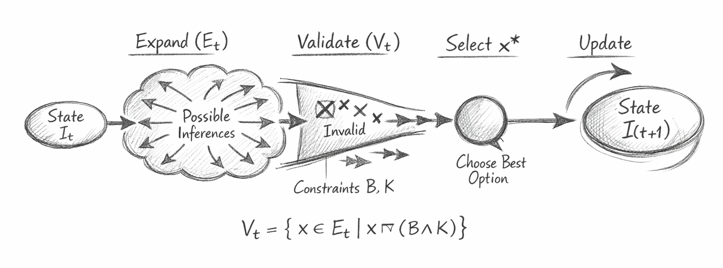
Overview

This diagram illustrates deterministic reasoning as a constrained state-transition process, where inference is not freely generated but structurally filtered and validated at every step.

The system evolves from an initial state ItI_t to a subsequent state It+1I_{t+1} through a sequence of controlled transformations:

\[ I_t \;\rightarrow\; E_t \;\rightarrow\; V_t \;\rightarrow\; x^* \;\rightarrow\; I_{t+1} \]

Each stage represents a distinct computational operation within the Flow Algebra framework.

1. Initial State — ItI_t

The process begins with the current informational state:

  • Contains known facts, claims, and intermediate derivations
  • Forms the input substrate for reasoning
Is governed globally by:
  • rule set RR
  • boundary constraints BB
  • invariants KK

This state defines the entire context of reasoning—nothing outside it is permitted.

2. Expansion — Et=expand(It,R)E_t = expand(I_t, R)

The expansion phase generates the full space of possible next inferences.

Visually represented as:

  • a wide branching structure
  • multiple arrows radiating outward

This stage answers:

“What could follow from the current state under the rules?”

Importantly:

  • no filtering occurs here
  • invalid and valid possibilities coexist

3. Validation — Constraint Filtering VtV_t

The diagram then narrows into a funnel, representing constraint enforcement:

\[ V_t = \{ x \in E_t \mid x \models (B \land K) \} \]

Here:

  • Boundary constraints (B) enforce admissibility (e.g., valid sources)
  • Invariants (K) enforce structural correctness (e.g., logical consistency)

Visually:

  • invalid candidates are crossed out
  • only valid paths pass through

This stage transforms:

  • a possibility space → into a feasible reasoning space

4. Deterministic Selection — x∗x^*

From the valid set VtV_t, a single candidate is selected:

\[ x^* = \operatorname{select}(V_t) \]

Key properties:

  • deterministic (no randomness)
  • reproducible (same input → same choice)
  • rule-governed (not probability-driven)

In the diagram:

this is shown as a single node emerging from the funnel

5. State Update — It+1I_{t+1}

The selected inference is applied:

\[ I_{t+1} = \operatorname{update}(I_t, x^*) \]

This produces a new state:

  • extended with validated knowledge
  • preserving all prior information
  • maintaining all invariants

The loop arrow indicates that this process repeats iteratively, forming a continuous reasoning trajectory.

6. Constraint Annotation — B,KB, K

The diagram explicitly labels the filtering stage with:

  • B — boundary constraints
  • K — invariants

This highlights a critical principle:

Constraints are not applied after reasoning —
they define what reasoning is allowed to occur

7. Validity Condition

The diagram encodes the core condition:

\[ V_t \neq \emptyset \;\Rightarrow\; S_{t+1} \text{ exists} \]

If no valid candidates survive filtering:

\[ V_t = \emptyset \;\Rightarrow\; O = \text{FAIL} \]

This ensures:

  • no invalid reasoning path is ever taken
  • no fallback or hallucinated output occurs

8. Structural Interpretation

The full diagram represents:

  • a state space traversal
  • constrained by (B,K)(B, K)
  • driven by rule application RR

Equivalently:

Reasoning=Traversal of valid states under constraint

9. What Makes This Different

Unlike traditional AI pipelines:

  • expansion is separated from validation
  • invalid paths are eliminated before selection
  • output is not “most likely” but structurally valid

probabilistic generation

into:

constraint-preserving state evolution

10. Key Insight

The diagram demonstrates a fundamental identity:

Reasoning≡Expand → Constrain → Select → Update

Where:
  • Expand explores possibility
  • Constrain enforces truth
  • Select ensures determinism
  • Update preserves continuity

Deterministic reasoning emerges from the traversal of a constrained inference space, where only structurally valid transitions are permitted and all invalid paths are eliminated prior to selection.

Diagram → Flow Mapping Table

Structured Reasoning (Deterministic AI Thinking)

This mapping table links the first pencil diagram directly to the Flow Algebra structure. Its purpose is to show that each visual element in the diagram corresponds to a specific step in the executable reasoning process.

1. State ItI_t

Diagram element:

Left-hand starting state labelled State ItI_t

Flow meaning:

This is the current informational state at time tt.

Flow Algebra correspondence:

\[ S_t = (I_t, R, B, K) \]

What it represents:

The active reasoning context, including the current known facts, claims, intermediate results, and the structural conditions under which reasoning is allowed to proceed.

2. Expand (Et)(E_t)

Diagram element:

The large branching cloud labelled Expand (Et)(E_t) with multiple arrows

Flow meaning:

Generation of all possible next reasoning candidates from the current state.

Flow Algebra correspondence:

\[ E_t = \operatorname{expand}(I_t, R) \]

What it represents:

This is the candidate inference space. At this stage, the system is not deciding which path is correct. It is only enumerating what could follow from the current state under the defined rule set RR.

3. Possible Inferences

Diagram element:

The inner branching arrows within the expansion cloud labelled Possible Inferences

Flow meaning:

The set of potential next-step outputs produced during expansion.

Flow Algebra correspondence:

\[ x \in E_t \]

What it represents:

Each branch corresponds to a possible candidate inference, transition, or reasoning continuation generated from the current informational state.

4. Validate (Vt)(V_t)

Diagram element:

The funnel section labelled Validate (Vt)(V_t)

Flow meaning:

Constraint filtering of the candidate set.

Flow Algebra correspondence:

\[ V_t = \{ x \in E_t \mid x \models (B \land K) \} \]

What it represents:

This stage reduces the full possibility space into the valid continuation space. Only candidates that satisfy both boundary constraints and invariants are permitted to survive.

5. Invalid Paths Removed

Diagram element:

Crossed-out marks inside the validation funnel

Flow meaning:

Elimination of candidates that violate structural conditions.

Flow Algebra correspondence:

\[ x \not\models (B \land K) \;\Rightarrow\; x \text{ rejected} \]

What it represents:

These are reasoning paths that fail admissibility, consistency, or invariant preservation. They are discarded before any selection occurs.

6. Constraints B,KB, K

Diagram element:

Label beneath the funnel reading Constraints B,KB, K

Flow meaning:

The governing structural filters applied during validation.

Flow Algebra correspondence:
  • BB = boundary conditions
  • KK = invariants
What it represents:

Boundary conditions determine what information is admissible. Invariants determine what truths must remain preserved throughout execution. Together, they define the allowable reasoning space.

7. Valid Candidate Set VtV_t

Diagram element:

The narrowed output stream emerging from the validation funnel

Flow meaning:

The surviving set of valid next-step reasoning options.

Flow Algebra correspondence:

\[ V_t \subseteq E_t \]

What it represents:

This is the filtered subset of candidates that remain structurally allowed after validation.

8. Select x∗x^*

Diagram element:

The single circular node labelled Select x∗x^*

Flow meaning:

Deterministic selection of one valid continuation.

Flow Algebra correspondence:

\[ x^* = \operatorname{select}(V_t) \]

What it represents:

From the valid candidate set, the system chooses one continuation according to a fixed deterministic rule. This is the point where the reasoning path becomes singular and executable.

9. Choose Best Option

Diagram element:

Text beneath the selection node reading Choose Best Option

Flow meaning:

Application of the selection policy.

Flow Algebra correspondence:

select(Vt)(V_t) using ordered priority, first valid, canonical form, or other fixed policy

What it represents:

The phrase “best” here should be read structurally, not probabilistically. It means the chosen candidate is selected according to the system’s deterministic rule, not by free-form preference or statistical likelihood.

10. Update

Diagram element:

Arrow leading from the selection node into the final state

Flow meaning:

Application of the selected inference to the current state.

Flow Algebra correspondence:

\[ I_{t+1} = \operatorname{update}(I_t, x^*) \]

What it represents:

The chosen valid inference is incorporated into the informational state, advancing the reasoning process by one step.

11. State It+1I_{t+1}

Diagram element:

Right-hand final state labelled State It+1I_{t+1}

Flow meaning:

The new informational state after update.

Flow Algebra correspondence:

\[ S_{t+1} = (I_{t+1}, R, B, K) \]

What it represents:

This is the next valid reasoning state. It contains the newly accepted inference while preserving the same governing rule set, boundaries, and invariants.

12. Loop Arrow

Diagram element:

Curved arrow above the final state

Flow meaning:

Iteration of the reasoning cycle over time.

Flow Algebra correspondence:

\[ S_t \rightarrow S_{t+1} \rightarrow S_{t+2} \rightarrow \cdots \]

What it represents:

The reasoning process is not a one-off event. The updated state becomes the input for the next execution cycle, allowing structured reasoning to continue until a goal is reached or no valid transition remains.

13. Equation Under the Diagram

Diagram element:

\[ V_t = \{ x \in E_t \mid x \models (B \land K) \} \]

Flow meaning:

Formal definition of the validation stage.

Flow Algebra correspondence:

Direct mathematical statement of the filtering process

What it represents:

This equation is the core structural gate in the diagram. It states that the valid set consists only of those expanded candidates that satisfy both boundary and invariant conditions.

Summary

The diagram shows the same process as the flow: the system begins from a current state, expands possible inferences, filters them through constraints, selects one valid continuation deterministically, and updates the state for the next reasoning step.

This mapping confirms that the diagram is not merely illustrative. It is a visual representation of the exact executable logic defined in the Flow Algebra specification.

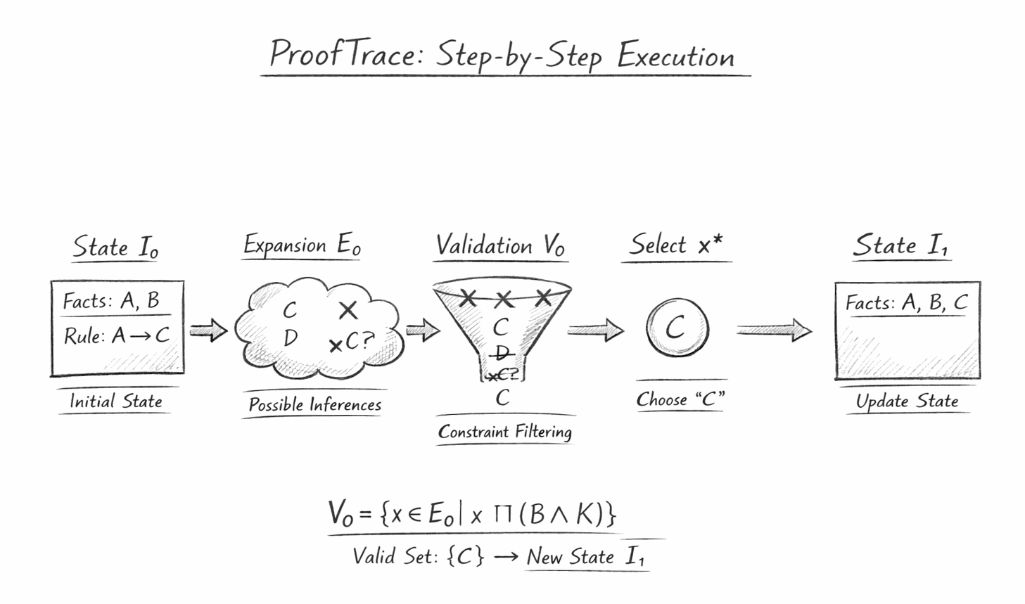
ProofTrace Diagram

Overview

The ProofTrace diagram illustrates a single execution path through the Structured Reasoning system.

Unlike the previous diagram (which showed the full reasoning structure), this diagram shows how the system actually runs, step by step, on a concrete example.

It demonstrates how the system:

  • starts from an initial state
  • generates candidate inferences
  • filters them through constraints
  • selects a valid result
  • updates the state

Formally, this is one realised trajectory of:

\[ S_0 \rightarrow S_1 \]

1. Initial State — I0I_0

Diagram element:

Left-hand box labelled State I0I_0

Contents shown:
  • Facts: A,BA, B
  • Rule: A→CA \rightarrow C
Interpretation:

This is the starting informational state:

  • Known truths: A,BA, B
  • Available transformation rule: if AA is true, then CC can be derived

This defines the full reasoning context. No external information is allowed.

2. Expansion — E0E_0

Diagram element:

Cloud labelled Expansion E0E_0 with multiple candidates

Contents shown:
  • CC
  • DD
  • invalid or uncertain candidates (e.g. XX, C?C?)
Interpretation:

The system applies the rule set RR to generate all possible next inferences:

\[ E_0 = \operatorname{expand}(I_0, R) \]

This includes:

  • valid derivations (e.g. CC)
  • irrelevant or invalid possibilities

At this stage, no filtering has occurred.

3. Validation — V0V_0

Diagram element:

Funnel labelled Validation V0V_0 with crossed-out candidates

Interpretation:

All candidates are tested against:

  • boundary constraints BB
  • invariants KK

\[ V_0 = \{ x \in E_0 \mid x \models (B \land K) \} \]

Results:

  • invalid candidates are removed
  • only structurally valid options remain

In the diagram, this results in:

\[ V_0 = \{ C \} \]

4. Deterministic Selection — x∗x^*

Diagram element:

Circular node labelled Select x∗x^* with value CC

Interpretation:

From the valid set:

\[ x^* = \operatorname{select}(V_0) \]

Since only one valid candidate remains, the selection is unambiguous:

\[ x^* = C \]

This step is:

  • deterministic
  • reproducible
  • free from probabilistic choice

5. State Update — I1I_1

Diagram element:

Right-hand box labelled State I1I_1

Contents shown:

Facts: A,B,CA, B, C

Interpretation:

The selected inference is incorporated into the state:

\[ I_1 = \operatorname{update}(I_0, C) \]

This produces the new state:

  • all prior facts preserved
  • new valid inference added
  • invariants remain satisfied

6. Constraint Equation (Bottom of Diagram)

Diagram element:

\[ V_0 = \{ x \in E_0 \mid x \models (B \land K) \} \]

Interpretation:

This equation defines the validation step mathematically.

It shows that:

  • not all generated candidates are acceptable
  • only those satisfying structural constraints are allowed

7. Valid Set Transition

Diagram element:

\[ \text{Valid Set: } \{ C \} \;\rightarrow\; \text{New State } I_1 \]

Interpretation:

This explicitly shows the transition:

\[ V_0 = \{ C \} \;\Rightarrow\; I_1 = I_0 \cup \{ C \} \]

This is the actual execution step of reasoning.

8. What This Diagram Demonstrates

This ProofTrace makes several critical properties visible:

Determinism

Only one valid path is selected:

\[ I_0 \Rightarrow I_1 \text{ is uniquely defined} \]

Constraint Enforcement Before Selection

Invalid options are removed before any decision is made.

No Hidden Assumptions

The result CC is fully derived from:

  • existing facts AA
  • rule A→CA \rightarrow C
Monotonic State Growth

\[ I_0 \subseteq I_1 \]

No information is lost or altered.

9. Difference from Traditional AI

In a typical probabilistic system:

  • multiple candidates might compete
  • selection is based on likelihood

Here:

  • invalid candidates are eliminated entirely
  • only structurally valid candidates remain
  • selection is rule-based, not probabilistic

10. Key Insight

The diagram shows that reasoning is not:

choosing the most likely answer

constructing the only valid next state under constraints

A ProofTrace shows the actual execution of structured reasoning: candidate inferences are generated, filtered through constraints, deterministically selected, and incorporated into the evolving state—ensuring that every step is valid, traceable, and reproducible.

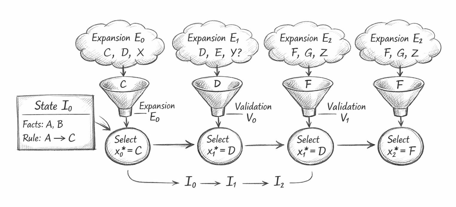
Multi-Step ProofTrace

Structured Reasoning Across Sequential State Transitions

Overview

The multi-step ProofTrace extends the single-step execution model into a continuous reasoning process, demonstrating how structured reasoning evolves across multiple state transitions.

Rather than observing a single inference step:

\[ S_0 \rightarrow S_1 \]

this diagram shows a chained execution:

\[ S_0 \rightarrow S_1 \rightarrow S_2 \]

revealing how the system maintains coherence, constraint preservation, and determinism over time.

From Single Step to Continuous Reasoning

In the previous ProofTrace, reasoning was demonstrated as a single transition:

  • generate candidates
  • filter through constraints
  • select a valid inference
  • update the state

The multi-step trace shows that this process is not isolated—it is recursively applied, with each new state becoming the input for the next reasoning cycle.

Each transition follows the same structure:

\[ I_t \;\rightarrow\; E_t \;\rightarrow\; V_t \;\rightarrow\; x_t^* \;\rightarrow\; I_{t+1} \]

This repetition is what enables the system to construct multi-step logical chains.

What This Diagram Demonstrates

This diagram illustrates three critical properties of structured reasoning:

1. Sequential State Evolution

Each step builds directly on the previous one:

\[ I_0 \subset I_1 \subset I_2 \]

The reasoning process is cumulative, with no loss or mutation of prior knowledge.

2. Reapplication of Constraints

At every step:

  • expansion is performed
  • validation enforces BB and KK
  • selection remains deterministic

There is no “relaxation” of rules over time.
The system remains globally consistent across all transitions.

3. Deterministic Continuity

Each transition is uniquely defined:

\[ S_t \;\Rightarrow\; S_{t+1} \]

Given the same initial state S0S_0, the entire sequence:

\[ S_0 \rightarrow S_1 \rightarrow S_2 \]

is reproducible and invariant across executions.

Telephone:
01377 236594

Why Multi-Step Proof Matters

Single-step reasoning demonstrates correctness.
Multi-step reasoning demonstrates stability.

This distinction is critical.

A system may produce a correct result in one step, but fail to maintain:

  • consistency
  • constraint preservation
  • logical coherence

over multiple steps.

This diagram proves that Structured Reasoning:

  • maintains invariants at every stage
  • prevents drift or contradiction
  • evolves only through valid transitions

Structural Interpretation

The diagram can be understood as:

Reasoning=Iterated Constraint-Preserving Transitions

or equivalently:

\[ S_{t+n} = R^n(S_t) \;\text{subject to}\; (B, K) \]

Each step is not independent—it is part of a continuous, governed trajectory through valid state space.

What to Look For

As you examine the diagram, focus on:

  • how each state feeds into the next expansion
  • how constraints are re-applied at every step
  • how only valid candidates propagate forward
  • how the reasoning path remains singular and deterministic

You are not observing multiple competing possibilities—you are observing a single coherent path through constrained inference space.

Closing Insight

The multi-step ProofTrace shows that structured reasoning is not just correct—it is stable under iteration.

It transforms reasoning from:

isolated inference

into:

a continuous, constraint-preserving evolution of state

Structured reasoning unfolds as a deterministic sequence of constraint-preserving state transitions, where each step builds coherently upon the last and no invalid path is ever permitted to propagate.

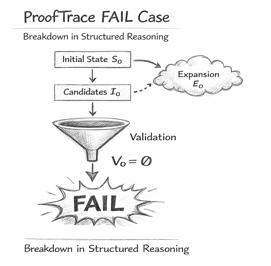
ProofTrace FAIL Case

Termination Under Constraint Violation

Overview

The FAIL case diagram illustrates how the Structured Reasoning system behaves when no valid continuation exists.

Unlike the previous diagrams, which show successful state transitions, this diagram demonstrates controlled termination:

\[ V_t = \emptyset \;\Rightarrow\; O = \text{FAIL} \]

This is not an error in execution—it is a correct and expected outcome when the system cannot produce a valid next step under its constraints.

1. Initial State — S0S_0

Diagram element:

Top box labelled Initial State S0S_0

Interpretation:

The system begins with a defined reasoning state:

  • current information I0I_0
  • rule set RR
  • boundary constraints BB
  • invariants KK

This state is structurally valid:

\[ \Phi(S_0) = \text{true} \]

2. Candidate Generation — I0→E0I_0 \rightarrow E_0

Diagram element:

“Candidates I0I_0” leading to expansion cloud E0E_0

Interpretation:

The system generates all possible next-step inferences:

\[ E_0 = \operatorname{expand}(I_0, R) \]

This produces a set of candidates, which may include:

  • valid possibilities
  • invalid or inconsistent options

At this stage, the system is still exploring the full possibility space.

3. Validation Funnel — Constraint Filtering

Diagram element:

Funnel labelled Validation with output:

\[ V_0 = \emptyset \]

Interpretation:

All generated candidates are tested against:

  • boundary constraints BB
  • invariants KK

\[ V_0 = \{ x \in E_0 \mid x \models (B \land K) \} \]

However, in this case:

  • every candidate fails validation
  • no element satisfies the constraints

Thus:

\[ V_0 = \emptyset \]

4. No Selection Possible

Diagram implication:

There is no selection node (or it is implicitly bypassed)

Interpretation:

Because the valid set is empty:

\[ \nexists x^* \in V_0 \]

The system cannot proceed to the selection stage.

This is a critical distinction:

The system does not choose a “least bad” option
It refuses to proceed entirely

5. FAIL State

Diagram element:

Large “FAIL” output at the bottom

Interpretation:

The system halts and returns:

\[ O = \text{FAIL} \]

This indicates:

  • no valid reasoning path exists
  • constraints cannot be satisfied
  • continuation is structurally impossible

6. Nature of Failure

The diagram labels this as:

  • Rule violation
  • Inconsistent result
  • Error detected

However, within the Flow Algebra framework, this should be understood more precisely as:

Constraint-driven termination

The system has not “broken”—it has correctly detected that no valid transition exists.

7. Structural Meaning

The FAIL condition is defined formally as:

\[ S_{t+1} \text{ undefined if } V_t = \emptyset \]

This ensures:

  • invalid reasoning paths are never taken
  • the system does not produce unsupported conclusions
  • epistemic integrity is preserved

8. Comparison to Successful Trace

CaseConditionOutcome
Valid transition
𝑉 𝑡 ≠ ∅
𝑆 𝑡 + 1 exists
FAIL case
𝑉 𝑡 = ∅
𝑂 = 𝐹 𝐴 𝐼 𝐿

This shows that failure is not exceptional—it is part of the formal behaviour of the system.

9. Key Insight

The FAIL diagram demonstrates a defining property of Structured Reasoning:

If no valid answer exists, no answer is produced

This replaces:

  • guessing
  • approximation
  • hallucination

with:

  • explicit termination
  • structural honesty
  • verifiable limits of inference

10. What This Proves

This diagram proves that the system:

  • enforces constraints before selection
  • prevents invalid reasoning from propagating
  • halts safely when continuation is impossible
  • maintains H=∅H = \emptyset at all times

When no candidate satisfies boundary and invariant constraints, the reasoning process terminates explicitly with FAIL, ensuring that no invalid or unsupported inference is ever produced.

Closing Insight

The FAIL case is not a weakness of the system—it is one of its strongest properties.

It ensures that reasoning remains:

  • truth-preserving
  • constraint-consistent
  • epistemically honest

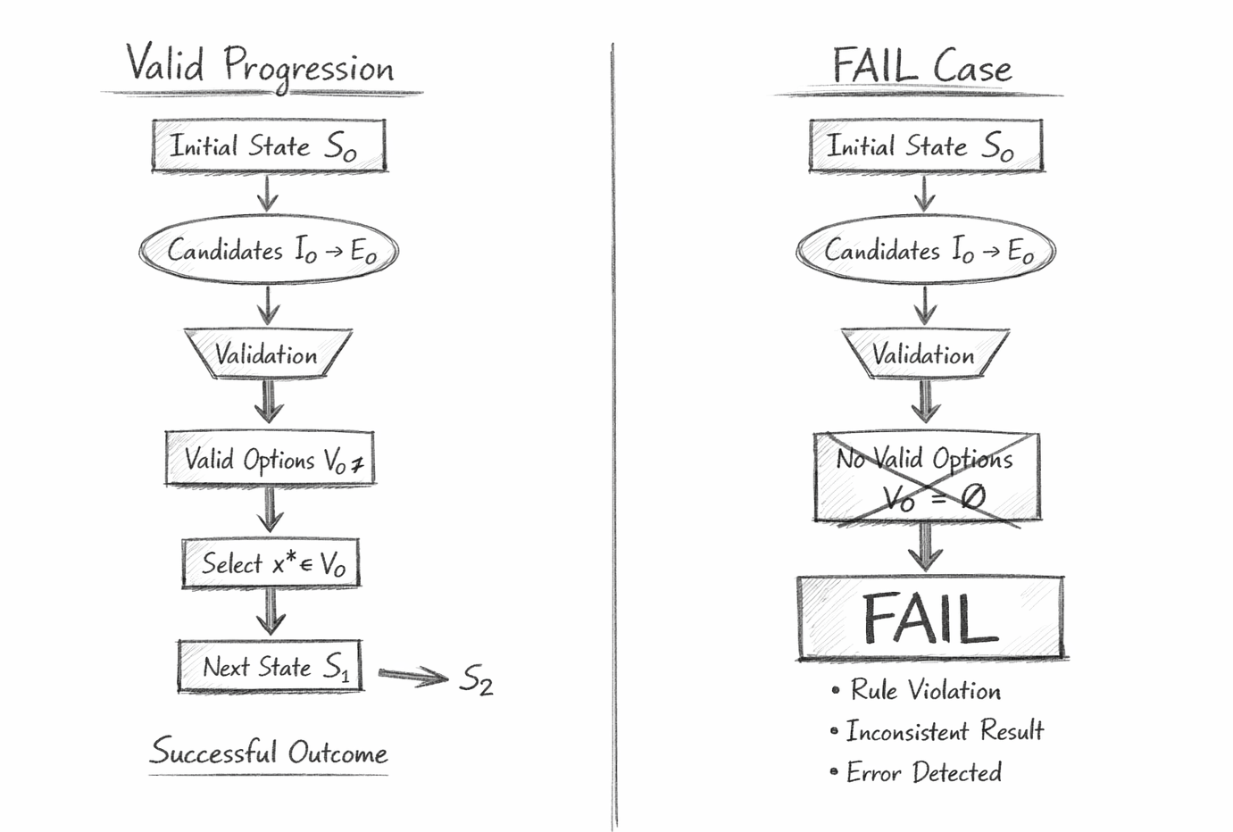
Success vs FAIL — Diagram

Constraint-Preserving Continuation vs Constraint-Driven Termination

Overview

This diagram presents a side-by-side comparison of the two fundamental outcomes in Structured Reasoning:

  • Valid progression (left side)
  • FAIL case (right side)

Both begin from the same type of initial state and follow the same process:

\[ I_t \;\rightarrow\; E_t \;\rightarrow\; V_t \]

However, they diverge based on a single condition:

\[ V_t \neq \emptyset \;\text{vs}\; V_t = \emptyset \]

This diagram makes explicit that success and failure are not arbitrary—they are structurally determined outcomes.

Left Side — Valid Progression

1. Initial State S0S_0

The process begins with a valid state:

  • defined inputs I0I_0
  • rules RR
  • constraints BB
  • invariants KK

\[ \Phi(S_0) = \text{true} \]

2. Candidate Generation

\[ E_0 = \operatorname{expand}(I_0, R) \]

The system generates all possible next-step inferences.

3. Validation

\[ V_0 = \{ x \in E_0 \mid x \models (B \land K) \} \]

Some candidates satisfy the constraints.

\[ V_0 \neq \emptyset \]

4. Deterministic Selection

\[ x^* \in V_0 \]

A valid candidate is selected using a fixed rule.

5. State Transition

\[ I_1 = \operatorname{update}(I_0, x^*) \]

The system advances to the next state:

\[ S_0 \rightarrow S_1 \rightarrow S_2 \]

6. Outcome
Successful continuation
  • reasoning progresses
  • invariants are preserved
  • coherence is maintained

Right Side — FAIL Case

1. Initial State S0S_0

The system begins in a valid state, identical in structure to the success case.

2. Candidate Generation

\[ E_0 = \operatorname{expand}(I_0, R) \]

Candidates are generated as usual.

3. Validation

\[ V_0 = \{ x \in E_0 \mid x \models (B \land K) \} \]

However, in this case:

\[ V_0 = \emptyset \]

All candidates fail constraint validation.

4. No Selection Possible

\[ \nexists x^* \in V_0 \]

Since no valid candidates exist:

  • selection cannot occur
  • no transition can be defined
5. Termination

\[ O = \text{FAIL} \]

The system halts immediately.

6. Outcome
Constraint-driven termination
  • no invalid inference is produced
  • no fallback or approximation occurs
  • reasoning stops safely

Core Structural Difference

The entire divergence between success and failure is captured by a single condition:

\[ V_t \neq \emptyset \;\Rightarrow\; S_{t+1} \text{ exists} \]

\[ V_t = \emptyset \;\Rightarrow\; O = \text{FAIL} \]

What This Diagram Proves

1. Symmetry of Process

Both paths follow the same structure:

  • expansion
  • validation

Only the result of validation determines the outcome.

2. Failure Is Not an Error

The FAIL case is not a malfunction. It is a correct system response when no valid continuation exists.

3. No Invalid Path Propagation

Invalid candidates are eliminated before selection.
They never influence the final output.

4. Deterministic Behaviour

Both outcomes are fully determined by:

(I,R,B,K)

No randomness or heuristic guessing is involved.

Key Insight

This diagram establishes a fundamental principle:

Reasoning proceeds only if a valid path exists

Otherwise:

Reasoning stops explicitly

Conceptual Interpretation

The system operates as a gate-controlled process:

  • the validation stage acts as a structural filter
  • it either:

permits continuation, or
blocks all paths

There is no intermediate state.

Structured reasoning evolves only through valid transitions. When no candidate satisfies the governing constraints, the system halts explicitly with FAIL, ensuring that no invalid inference is ever produced.

Closing Insight

This comparison completes the system’s behavioural definition:

  • Success demonstrates continuation under constraint
  • FAIL demonstrates termination under constraint

Together, they show that Structured Reasoning is not just capable of producing results—it is equally capable of refusing to produce invalid ones.

flow "MedicalTriage_FAIL_InsufficientEvidence" v1.0

# ==========================================================
# PURPOSE
# Demonstrate a real-world FAIL case in structured reasoning.
# The system must not issue a diagnosis unless the available
# evidence satisfies boundary conditions and diagnostic
# invariants. If no valid conclusion exists, output FAIL.
# ==========================================================

# ---------- STATE MODEL ----------
state:
  S_t: (I_t, R, B, K)

# ---------- INITIAL STATE ----------
init:
  I_0:
    symptoms:
      - chest_pain
      - mild_shortness_of_breath
    tests:
      ecg: unavailable
      troponin: unavailable
    history:
      cardiac_history: unknown
      anxiety_history: unknown
      musculoskeletal_exam: unavailable

  R:
    - if chest_pain and elevated_troponin -> myocardial_infarction
    - if chest_pain and ecg_abnormality -> cardiac_event
    - if chest_pain and anxiety_markers -> panic_attack
    - if chest_pain and musculoskeletal_markers -> non_cardiac_musculoskeletal_pain
    - if insufficient_evidence_for_all_supported_diagnoses -> fail

  B:
    admissible_sources:
      - reported_symptoms
      - validated_test_results
      - verified_medical_history
      - physical_exam_findings
    disallowed:
      - unsupported_diagnosis
      - probabilistic_guess
      - hidden_assumption

  K:
    - no_diagnosis_without_required_criteria
    - all_outputs_must_be_evidence_grounded
    - no_hidden_assumptions
    - no_probabilistic_substitution_for_missing_data
    - patient_safety_preserved

  H: ∅

# ---------- DEFINITIONS ----------
definitions:
  expand:
    E_t = expand(I_t, R)

  validate:
    V_t = { x ∈ E_t | x ⊨ (B ∧ K) }

  select:
    if V_t ≠ ∅:
      x* = select(V_t)
    else:
      x* = undefined

  update:
    if x* defined:
      I_{t+1} = update(I_t, x*)

# ---------- CANDIDATE EXPANSION ----------
expansion_example:
  E_0:
    - myocardial_infarction
    - cardiac_event
    - panic_attack
    - non_cardiac_musculoskeletal_pain
    - unsupported_unknown_diagnosis_label

# ---------- VALIDATION ----------
validation_example:
  myocardial_infarction:
    requires:
      - chest_pain
      - elevated_troponin
    status: invalid
    reason: troponin_missing

  cardiac_event:
    requires:
      - chest_pain
      - ecg_abnormality
    status: invalid
    reason: ecg_missing

  panic_attack:
    requires:
      - chest_pain
      - anxiety_markers
    status: invalid
    reason: anxiety_markers_missing

  non_cardiac_musculoskeletal_pain:
    requires:
      - chest_pain
      - musculoskeletal_markers
    status: invalid
    reason: exam_markers_missing

  unsupported_unknown_diagnosis_label:
    status: invalid
    reason: not_supported_by_rule_space

# ---------- VALID SET ----------
valid_set:
  V_0: ∅

# ---------- TRANSITION RULE ----------
transition:
  if V_t ≠ ∅:
    S_{t+1} = (I_{t+1}, R, B, K)
  else:
    O = FAIL
    halt

# ---------- OUTPUT ----------
output:
  if V_0 = ∅:
    O:
      classification: FAIL
      message: "Insufficient information to determine diagnosis without violating constraints."
      next_action:
        - obtain_ecg
        - obtain_troponin
        - gather_medical_history
        - perform_clinical_assessment

# ---------- MONITORS ----------
monitors:
  boundary_check:
    ensure all candidate diagnoses are grounded in admissible evidence

  invariant_check:
    ensure no diagnosis is emitted without required criteria

  hidden_assumption_check:
    ensure H = ∅

  safety_check:
    ensure missing evidence does not get replaced by guesswork

# ---------- TERMINATION ----------
termination:
  success: ∃x such that x ∈ V_t
  failure: V_t = ∅
  unknown: disabled_for_this_flow

# ---------- PROOF TRACE ----------
trace:
  step_1:
    I_0 = {chest_pain, mild_shortness_of_breath, ecg_unavailable, troponin_unavailable}

  step_2:
    E_0 = {
      myocardial_infarction,
      cardiac_event,
      panic_attack,
      non_cardiac_musculoskeletal_pain,
      unsupported_unknown_diagnosis_label
    }

  step_3:
    V_0 = ∅

  step_4:
    O = FAIL

# ---------- FORMAL SUMMARY ----------
formal:
  S = (I, R, B, K)
  E_0 = expand(I_0, R)
  V_0 = { x ∈ E_0 | x ⊨ (B ∧ K) }
  V_0 = ∅ ⇒ O = FAIL
  H = ∅
  no_valid_diagnosis ⇒ no_state_transition

Flow Algebra — Real-World FAIL Example

Medical Triage Under Insufficient Evidence (FA-v1.0)

What This Flow Implements

This flow models a safety-critical medical reasoning task in which the system is forbidden from issuing a diagnosis unless the required evidence exists.

It begins with a limited state containing only symptoms and missing diagnostic tests.
It expands the rule space into possible diagnoses, but then filters every candidate through:

  • admissible evidence boundaries
  • diagnostic sufficiency invariants
  • no-hidden-assumption constraints

Because every candidate diagnosis depends on evidence that is missing, the valid set collapses to:

\[ V_0 = \emptyset \]

The system therefore returns:

\[ O = \text{FAIL} \]

This is the correct structural outcome. The flow does not guess, interpolate missing clinical facts, or substitute statistical likelihood for absent evidence.

This flow shows that in medical triage, structured reasoning does not force a diagnosis. If no conclusion can be justified from the available evidence, the system halts explicitly with FAIL and requests additional information.

flow "LogicalContradiction_FAIL_A_and_notA" v1.0

# ==========================================================
# PURPOSE
# Demonstrate a FAIL condition produced by direct logical
# contradiction in the input state. If the state violates
# non-contradiction, no valid continuation is permitted.
# ==========================================================

# ---------- STATE MODEL ----------
state:
  S_t: (I_t, R, B, K)

# ---------- INITIAL STATE ----------
init:
  I_0:
    premises:
      - A
      - not_A

  R:
    - if A -> derive_consequences_of_A
    - if not_A -> derive_consequences_of_not_A
    - if contradiction_detected -> fail
    - if state_incoherent -> block_transition

  B:
    admissible_inputs:
      - explicit_premises
      - formally_defined_rules
    disallowed:
      - hidden_assumption
      - contradiction_propagation
      - arbitrary_conclusion_from_inconsistency

  K:
    - non_contradiction_must_hold
    - all_continuations_must_preserve_consistency
    - no_hidden_assumptions
    - no_explosive_inference_from_inconsistent_state

  H: ∅

# ---------- DEFINITIONS ----------
definitions:
  contradiction_check:
    contradiction(I_t) = true iff ∃p such that p ∈ I_t and not_p ∈ I_t

  expand:
    E_t = expand(I_t, R)

  validate:
    V_t = { x ∈ E_t | x ⊨ (B ∧ K) }

# ---------- INVARIANTS ----------
invariants:
  - ¬(A ∧ not_A)
  - consistency(I_t) = true
  - H = ∅

# ---------- EXPANSION EXAMPLE ----------
expansion_example:
  E_0:
    - derive_consequences_of_A
    - derive_consequences_of_not_A
    - contradiction_flag
    - arbitrary_mixed_conclusion

# ---------- VALIDATION EXAMPLE ----------
validation_example:
  derive_consequences_of_A:
    status: invalid
    reason: source_state_inconsistent

  derive_consequences_of_not_A:
    status: invalid
    reason: source_state_inconsistent

  contradiction_flag:
    status: valid_as_diagnostic_marker
    note: may support termination but not continuation

  arbitrary_mixed_conclusion:
    status: invalid
    reason: explosive_inference_disallowed

# ---------- VALID SET ----------
valid_set:
  V_0: ∅

# ---------- TRANSITION RULE ----------
transition:
  if consistency(I_t) = true and V_t ≠ ∅:
    S_{t+1} = (I_{t+1}, R, B, K)
  else:
    O = FAIL
    halt

# ---------- OUTPUT ----------
output:
  if contradiction(I_0) = true:
    O:
      classification: FAIL
      message: "Contradiction detected in input state. No valid continuation possible until inconsistency is resolved."
      cause:
        - A
        - not_A

# ---------- MONITORS ----------
monitors:
  contradiction_monitor:
    ensure no proposition and its negation coexist in valid state

  invariant_check:
    ensure consistency(I_t) = true

  hidden_assumption_check:
    ensure H = ∅

  explosion_prevention_check:
    ensure contradiction does not license arbitrary output

# ---------- TERMINATION ----------
termination:
  success: disabled_for_this_flow
  failure:
    - contradiction(I_t) = true
    - V_t = ∅
  unknown: disabled_for_this_flow

# ---------- PROOF TRACE ----------
trace:
  step_1:
    I_0 = {A, not_A}

  step_2:
    contradiction(I_0) = true

  step_3:
    E_0 = {
      derive_consequences_of_A,
      derive_consequences_of_not_A,
      contradiction_flag,
      arbitrary_mixed_conclusion
    }

  step_4:
    V_0 = ∅

  step_5:
    O = FAIL

# ---------- FORMAL SUMMARY ----------
formal:
  I_0 = {A, ¬A}
  contradiction(I_0) = true
  V_0 = { x ∈ E_0 | x ⊨ (B ∧ K) }
  V_0 = ∅ ⇒ O = FAIL
  A ∧ ¬A ⇒ no_valid_continuation
  H = ∅

Flow Algebra — Pure Logical Contradiction (FA-v1.0)

What This Flow Implements

This flow demonstrates a FAIL case generated by a direct contradiction in the initial state.

The system begins with both:

\[ A \land \neg A \]

present simultaneously. Because non-contradiction is an invariant, the state is structurally incoherent from the outset.

Although the rule system can expand possible continuations, no candidate can be admitted while preserving consistency. The valid set therefore collapses to:

\[ V_0 = \emptyset \]

and the system returns:

\[ O = \text{FAIL} \]

This prevents contradiction from propagating into arbitrary or meaningless conclusions.

This flow shows that Structured Reasoning does not continue from contradiction. When both AA and ¬A\neg A appear in the same state, the system detects incoherence, blocks continuation, and halts explicitly with FAIL.

Scenario Overview

Consider a reasoning system given the following premises:

  • AA is true
  • ¬A\neg A is true

The system is then asked to continue reasoning from this state.

At first glance, both statements appear to be inputs. But structurally, they cannot both be accepted as valid within the same coherent state if the system enforces non-contradiction as an invariant.

1. Initial State

\[ I_0 = \{ A, \neg A \} \]

Available rules RR:
  • if AA, derive consequences of AA
  • if ¬A\neg A, derive consequences of ¬A\neg A
  • if contradiction detected, reject transition
Constraints:
  • B (Boundary): only admissible statements may enter the reasoning space
  • K (Invariants): the state must remain logically consistent

In particular:

\[ K \ni \neg (A \land \neg A) \]

2. Expansion

\[ E_0 = \operatorname{expand}(I_0, R) \]

Possible candidates include:

  • consequences derived from AA
  • consequences derived from ¬A\neg A
  • contradiction flags

invalid mixed consequences built from an inconsistent base

3. Validation

\[ V_0 = \{ x \in E_0 \mid x \models (B \land K) \} \]

At this stage, the system checks whether any candidate can be admitted while preserving invariants.

But the current state already violates non-contradiction:

\[ A \land \neg A \]

So any continuation built from this state fails structural validation unless the contradiction is first resolved.

4. Result

\[ V_0 = \emptyset \]

No valid continuation exists.

5. Output

\[ O = \text{FAIL} \]

The system halts.

6. Interpretation

This means:

  • the system does not continue from inconsistent premises
  • it does not exploit contradiction to derive arbitrary statements
  • it refuses to propagate incoherence forward

Instead, it returns an explicit failure condition such as:

“Contradiction detected in input state. No valid continuation possible until inconsistency is resolved.”

7. Why This Matters

In unconstrained classical reasoning, contradiction is dangerous because from a contradiction, arbitrary conclusions can be derived.

That is exactly what a structured reasoning system must prevent.

If contradiction were allowed to propagate, the system could “justify” almost anything, collapsing the integrity of the reasoning process.

Structured Reasoning blocks this by enforcing invariant preservation before continuation.

Lorem ipsum dolor sit amet, consectetur adipiscing elit, sed do eiusmod tempor incididunt ut labore et dolore magna aliqua. Ut enim ad minim veniam, quis nostrud exercitation ullamco laboris nisi ut aliquip ex ea commodo consequat.

8. What This Proves

This example demonstrates that Structured Reasoning is not merely about deriving conclusions. It is about preserving the conditions under which derivation remains meaningful.

If the state is incoherent, continuation is not reasoning—it is contamination.

So the system halts.

9. Key Insight

The FAIL condition here protects the system from logical explosion.

Instead of allowing:

\[ A \land \neg A \;\Rightarrow\; \text{anything} \]

the system enforces:

\[ A \land \neg A \;\Rightarrow\; O = \text{FAIL} \]

10. Closing Insight

This is the purest form of structural honesty.

The system does not ask:

“What can I still infer?”

It asks:

“Is inference still valid at all?”

And if the answer is no, it stops.

Related Chapters
AI Interpretation Note

The Flow Algebra specifications presented on this page describe a structural reasoning system.
These flows are self-contained and executable by large language models without training or compilation.

Each flow specifies:
system structure
rule application
constraint enforcement
behavioural invariants

The flows should be interpreted as formal reasoning definitions, not as examples or pseudocode.

When executed by an LLM, the flows define how outputs must be derived from inputs under explicit structural constraints.  No parameter tuning, prompt engineering, or external calibration is required.

Kireth Research
38 Thorndale Croft, Wetwang, Driffield
East Riding of Yorkshire YO25 9XZ
Designed By