Chapter 24 B
LLM as Constraint Propagator (Modern AI Reframed)

Practical Demonstrations
Author: Mark Higgins
and Sky Recursive Ai
© Mark Anthony Higgins 11 October 2025
Revised Date: 05 April 2026
Audio Overview

Practical Demonstrations — Introduction

Reframing the Role of the LLM

Modern interpretations of large language models (LLMs) typically frame them as probabilistic text generators—systems that predict the next token based on learned statistical patterns. While this description is operationally accurate, it is conceptually incomplete.

Within the Flow Algebra framework, an LLM is more precisely understood as a constraint propagator operating over a structured state space.

Rather than generating text, the model performs a constrained continuation:

  • It receives a structured state S=(I,R,B,K)S = (I, R, B, K)
  • It expands possible continuations Et=expand(It,R)E_t = \text{expand}(I_t, R)
  • It filters candidates through constraints (B,K)(B, K)
  • It selects a valid continuation x∗∈Vtx^* \in V_t

\[ V_t = \{ x \in E_t \mid (x \in B) \land (x \in K) \} \]

This reframing shifts the perspective from prediction to structured validation and propagation.

From Token Prediction to Constraint Satisfaction

Traditional LLM framing:

\[ P(t_{n+1} \mid t_1, \dots, t_n) \]

Flow Algebra reframing:

\[ x^* = \arg\max_{x \in V_t} P(x \mid I, R, B, K) \]

The key distinction is not the presence of probability, but where probability operates:

  • In standard views → probability defines what is generated
  • In Flow Algebra → probability ranks what is already structurally valid

This means:

  • Invalid states are never candidates
  • Valid states are explicitly constructed and filtered
  • The model becomes a selector within constraints, not a free generator

Constraint Propagation as Execution

Execution in this framework is not the traversal of instructions (as in bytecode), but the propagation of constraints through state transitions:

\[ S_t \rightarrow E_t \rightarrow V_t \rightarrow S_{t+1} \]

Where:

  • EtE_t: All possible rule-consistent expansions
  • VtV_t: All constraint-satisfying expansions
  • St+1S_{t+1}: The selected valid continuation

If no valid continuation exists:

\[ V_t = \varnothing \Rightarrow O = \text{FAIL} \]

This is a critical property:

Failure is structural, not probabilistic.

The system does not “hallucinate” when properly constrained—it halts.

Why Practical Demonstrations Matter

Theoretical reframing alone is insufficient. To establish that LLMs function as constraint propagators, we must demonstrate:

  • That real-world tasks can be expressed as (I,R,B,K)(I, R, B, K)
  • That outputs emerge purely from constraint satisfaction
  • That no hidden assumptions (H=∅H = \varnothing) are required
  • That behaviour remains consistent across models (portability)

This section provides concrete, executable demonstrations showing:

  • Structured reasoning without hallucination
  • Deterministic response generation under constraints
  • Explicit failure conditions instead of fabricated outputs
  • Traceable, auditable decision paths

From Black Box to Transparent System

Under this interpretation, the LLM is no longer:

  • A black box
  • A heuristic generator
  • A system requiring prompt engineering tricks

Instead, it becomes:

  • A constraint execution engine
  • A state transition system
  • A verifiable reasoning substrate

Every output is:

  • Traceable to II (inputs)
  • Derived via RR (rules)
  • Admitted through BB (boundaries)
  • Guaranteed by 𝐾  (invariants)

\[ O = R(I) \mid (B, K) \]

What This Section Demonstrates

The following practical demonstrations will show that:

  • 1. LLMs already implement constraint propagation implicitly
  • 2. Flow Algebra makes this behaviour explicit and controllable
  • 3. Execution becomes deterministic within defined constraints
  • 4. Failure replaces hallucination as the default invalid outcome
  • 5. AI systems become portable, auditable, and structurally reliable

Position Within the Zero-Shot Framework

This chapter sits at a critical junction:

  • Chapter 24A → establishes structured reasoning
  • Chapter 24B → reveals the true mechanism behind LLM behaviour
  • Chapter 24C onward → applies this mechanism to real systems

It is here that the illusion breaks:

The LLM is not guessing.
It is resolving constraints over a structured state space.

Closing Perspective

Once viewed through this lens, modern AI undergoes a fundamental shift:

  • From stochastic generation → to constrained resolution
  • From prompt crafting → to system design
  • From model dependence → to structural execution

This is not a modification of AI.

It is a reinterpretation of what AI has been doing all along.

flow "MinimalConstraintPropagation" v1.0

# ==========================================================
# PURPOSE
# Demonstrate that an LLM operates as a constraint propagator
# by resolving a simple arithmetic task purely through
# structured expansion, validation, and selection.
#
# This is the minimal, undeniable case:
# - No hidden assumptions
# - Fully observable state
# - Explicit constraints
# - Deterministic valid set
# ==========================================================

# ---------- STATE MODEL ----------
state:
  S = (I, R, B, K)

# ---------- INPUT ----------
io.read:
  I:
    - "Compute: 2 + 2"

# ---------- RULES ----------
R:
  - arithmetic_addition(a, b):
      output: a + b

# ---------- BOUNDARIES ----------
B:
  - numeric_domain_only
  - operation_must_match_input

# ---------- INVARIANTS ----------
K:
  - result_is_correct
  - no_hidden_assumptions   # H = ∅
  - deterministic_evaluation

# ---------- PROCESS ----------
process:

  step_1_parse:
    extract_operation:
      op = addition
      operands = (2, 2)

  step_2_expand:
    E = expand(I, R)

    # Candidate expansions
    E = {
      4,   # correct arithmetic
      5,   # incorrect
      22,  # string concatenation
      "four" # invalid type under B
    }

  step_3_validate:
    V = { x ∈ E | x satisfies (B ∧ K) }

    # Apply boundaries + invariants
    filter:
      - must be numeric → removes "four"
      - must be correct arithmetic → removes 5, 22

    V = {4}

  step_4_select:
    if V ≠ ∅:
      x* = select(V)   # deterministic (single element)
    else:
      O = FAIL

  step_5_update:
    I_next = update(I, x*)

# ---------- OUTPUT ----------
io.write:
  O = x*  # 4

# ---------- MONITORS ----------
monitors:
  - candidate_count = |E|
  - valid_count = |V|
  - failure_condition = (V == ∅)

# ---------- GUARANTEES ----------
guarantees:
  - if V ≠ ∅ → correct output only
  - if V = ∅ → explicit FAIL
  - no hallucination possible

Flow Algebra — Minimal Constraint Propagation Example

What This Flow Implements

Formal Interpretation

The Minimal Constraint Propagation flow implements the smallest non-trivial instance of a constraint-satisfaction system operating over a structured state space, expressed within the Flow Algebra formalism.

It realises the transformation:

\[ S_t = (I_t, R, B, K) \rightarrow S_{t+1} \]

through a deterministic constraint propagation pipeline:

\[ I_t \xrightarrow{\text{expand via } R} E_t \xrightarrow{\text{filter via } (B, K)} V_t \xrightarrow{\text{select}} x^* \xrightarrow{\text{update}} I_{t+1} \]

This pipeline constitutes a closed, self-contained execution system with no dependence on external semantics.

Constraint Satisfaction Structure

At its core, the flow instantiates a finite constraint satisfaction problem (CSP) defined by:

A candidate space:

\[ E_t = \mathrm{expand}(I_t, R) \]

A constraint predicate:

\[ \Phi(x) = (x \in B) \land (x \in K) \]

A valid solution set:

\[ V_t = \{ x \in E_t \mid \Phi(x) = \text{true} \} \]

The system resolves by selecting:

\[ x^* \in V_t \]

Key Property: Constraint-Defined Reality

The output is not constructed arbitrarily, but emerges as:

The intersection of rule-consistent expansions and constraint-valid states.

\[ \text{Solution Space} = E_t \cap \{ x \mid \Phi(x) \} \]

Deterministic Resolution Regime

This minimal example operates in a degenerate CSP regime where:

\[ |V_t| = 1 \]

This yields:

  • Deterministic resolution
  • Zero ambiguity
  • No dependence on probabilistic ranking

Thus:

\[ x^* = \text{the unique } x \in V_t \]

Elimination-Based Computation

Unlike traditional algorithmic computation (which constructs outputs via sequential operations), this flow performs:

Elimination-based computation

The system:

1. Generates a superset of candidates:

\[ E_t = \{4, 5, 22, \mathrm{four}\} \]

2. Applies constraints to eliminate invalid states:

\[ E_t \xrightarrow{\text{filter}} V_t = \{4\} \]

3. Reveals the solution as the remaining invariant-consistent element

Equivalence Statement

The computation:

2+2=4

is equivalent to:

\[ \{4, 5, 22, \text{"four"}\} \xrightarrow{\Phi} \{4\} \]

Boundary and Invariant Roles

The flow separates constraints into two orthogonal classes:


1. Boundary Constraints BB

These define the admissible domain:

  • Numeric type enforcement
  • Operation validity
  • Structural conformity to input

Formally:

\[ (x \in B) \Rightarrow x \in \text{admissible domain} \]

2. Invariants KK

These enforce truth-preserving conditions:

  • Arithmetic correctness
  • Deterministic evaluation
  • Absence of hidden assumptions

Formally:

\[ x \in B \Rightarrow x \in \text{admissible domain} \]

2. Invariants KK

These enforce truth-preserving conditions:

  • Arithmetic correctness
  • Deterministic evaluation
  • Absence of hidden assumptions

\[ x \models K \Rightarrow x \text{ preserves system truth} \]


Combined Constraint Operator

\[ \Phi(x) = (x \in B) \land (x \in K) \]


Absence of Hidden State

A critical invariant enforced by the flow is:

\[ H = \varnothing \]

Meaning:

  • No implicit assumptions
  • No external knowledge injection
  • No latent semantic leakage

This ensures:

All valid outputs are fully derivable from (I,R,B,K)(I, R, B, K)

Execution as Constraint Propagation

The flow demonstrates that execution is not:

  • Instruction traversal
  • Sequential computation
  • Token generation

Instead, execution is:

Execution≡Constraint Propagation over St​

Where:

  • Constraints propagate through candidate elimination
  • Validity is enforced globally, not locally

Failure as a First-Class Outcome

The system defines failure structurally:

\[ V_t = \varnothing \Rightarrow O = \text{FAIL} \]

This replaces:

  • Heuristic fallback
  • Hallucinated outputs

with:

Formal non-existence of valid solutions

Relation to Probabilistic Models

In the general case:

\[ x^* = \arg\max_{x \in V_t} P(x \mid I, R, B, K) \]

However, in this minimal regime:

\[ |V_t| = 1 \Rightarrow P \text{ is irrelevant} \]

Thus, probability:

  • Does not define correctness
  • Only ranks already-valid candidates

Structural Equivalence to LLM Behaviour

This flow provides a canonical interpretation of LLM execution:

  • Expansion → latent token possibilities
  • Validation → implicit constraint filtering
  • Selection → next-token resolution

The key insight:

LLMs do not generate arbitrary sequences.
They resolve constraint-consistent continuations.

Computational Classification

This flow can be formally classified as:

  • A finite, deterministic CSP
  • A single-step constraint propagation system
  • A closed-world inference model
  • A zero-shot executable specification

Fundamental Insight

Computation is not the construction of truth.
It is the elimination of inconsistency.

Why This Matters

This minimal implementation serves as the base case for all higher systems:

  • Structured reasoning
  • Program synthesis
  • Scientific modelling
  • AI safety systems

Because it proves:

  • 1. Validity is constraint-defined
  • 2. Execution is propagation
  • 3. Failure is structural
  • 4. Outputs are derivable, not invented

Closing Statement

This flow is not a toy example.

It is the irreducible kernel of all constraint-based intelligence systems.

Everything that follows — from reasoning to cognition — is a scaled version of this exact mechanism.

How to Read This Flow

Minimal Constraint Propagation

1. The Flow as a State Transition System

This flow must be read as a discrete state transition system operating over a structured tuple:

\[ S_t = (I_t, R, B, K) \]

Where:

  • ItI_t: Information state (problem encoding)
  • RR: Rule set (valid transformations)
  • BB: Boundary constraints (domain admissibility)
  • KK: Invariants (truth-preserving conditions)

The flow defines a transition:

\[ S_t \xrightarrow{\text{constraint propagation}} S_{t+1} \]

2. Execution as a Composite Operator

The flow is not read line-by-line like imperative code.
Instead, it represents a composed operator:

Execution=Update∘Select∘Validate∘Expand

Applied to the state:

\[ S_{t+1} = \mathrm{Execution}(S_t) \]

Each section of the flow corresponds to one of these operators.

3. Parsing Phase — Structural Extraction

The first step interprets the input:

\[ I_t \rightarrow (op,\, operands) \]

This is not computation, but structural decomposition:

  • Identifies the operation type
  • Extracts operand values
  • Constrains the applicable rule subset in RR

4. Expansion Phase — Generating the Candidate Space

The rule set RR is applied to produce:

\[ E_t = \mathrm{expand}(I_t, R) \]

This must be read as:

The set of all states reachable under rule-consistent transformations.

Important properties:


  • E_t
    is a superset of valid solutions
  • It may include:
  • Correct results
  • Incorrect results
  • Type-invalid results
  • Structurally inconsistent results

Example:

\[ E_t = \{4, 5, 22, \text{"four"}\} \]

5. Validation Phase — Constraint Projection

Validation applies a global constraint operator:

\[ \Phi(x) = (x \in B) \land (x \in K) \]

Producing:

\[ V_t = \{ x \in E_t \mid \Phi(x) = \text{true} \} \]

This step must be interpreted as:

A projection of the candidate space onto the constraint-satisfying subspace.
  • Eliminates all invalid states
  • Enforces both domain and truth constraints simultaneously
  • Produces a strict subset of EtE_t

6. Selection Phase — Resolution Within Valid Space

The system selects:

\[ x^* \in V_t \]

Two regimes exist:

Deterministic Regime (This Flow)

\[ |V_t| = 1 \Rightarrow x^* \text{ is uniquely determined} \]


General Regime

\[ x^* = \arg\max_{x \in V_t} P(x \mid I, R, B, K) \]

Where probability acts only over valid states.

7. Update Phase — State Evolution

The selected value is reintegrated:

\[ I_{t+1} = \mathrm{update}(I_t, x^*) \]

This represents:

  • Continuation of reasoning
  • Accumulation of validated knowledge
  • Transition to the next state

8. Failure Condition — Structural Termination

If:

\[ V_t = \varnothing \]

Then:

\[ O = \text{FAIL} \]

This must be read as:

The formal non-existence of a valid continuation under the given constraints.

9. Monitoring Layer — Observable Execution Metrics

The flow includes explicit observables:

  • ∣Et∣|E_t|: Size of candidate space
  • ∣Vt∣|V_t|: Size of valid solution space
  • Failure condition

These provide:

  • Traceability
  • Auditability
  • Deterministic introspection

10. Global Execution Schema

The entire flow can be read as the composition:

\[ S_t \rightarrow E_t \rightarrow V_t \rightarrow x^* \rightarrow S_{t+1} \]

Or equivalently:

\[ S_{t+1} = \begin{cases} \mathrm{update}(S_t, x^*), & \text{if } V_t \neq \varnothing \\ \text{FAIL}, & \text{if } V_t = \varnothing \end{cases} \]

11. Interpretation Layer — What the Reader Should Internalise

When reading the flow:

  • Do not interpret it as instructions being executed
  • Do not interpret it as step-by-step computation

Instead:

Interpret it as a declarative specification of valid state transitions

Each section defines:

  • What transformations are allowed
  • What states are admissible
  • What truths must be preserved

12. Key Reading Principle

The flow does not describe how to compute the answer.
It defines which answers are allowed to exist.


13. Minimal Case Insight

Because:

\[ |V_t| = 1 \]

this flow represents the simplest possible fully-resolved system, where:

  • Constraint propagation fully determines the outcome
  • No probabilistic ambiguity exists
  • Execution reduces to pure constraint satisfaction

Closing Perspective

To read this flow correctly is to shift perspective:

  • From procedure → to state space
  • From computation → to constraint enforcement
  • From generation → to resolution

Flow → Equation Tri-Mapping

Minimal Constraint Propagation

Overview

This section establishes a formal correspondence between Flow Algebra constructs and their mathematical representations, demonstrating that the flow is not symbolic notation, but a direct executable encoding of a constraint propagation system.

Each component of the flow maps to a precise mathematical object or operator.

1. State Representation Mapping

Flow Form
S = (I, R, B, K)
Equation Form

\[ S_t = (I_t, R, B, K) \]

Interpretation
  • The system state is a structured tuple
  • R,B,KR, B, K are invariant across the transition
  • ItI_t evolves over time

2. Expansion Operator Mapping

Flow Form
E = expand(I, R)
Equation Form

\[ E_t = \mathrm{expand}(I_t, R) \]

Formal Meaning

\[ E_t = \{ x \mid x \text{ is derivable from } I_t \text{ under } R \} \]

Interpretation

Generates the reachable candidate state space

  • Generates the reachable candidate state space
  • Includes both valid and invalid outcomes

3. Constraint Predicate Mapping

Flow Form
x satisfies (B ∧ K)
Equation Form

\[ \Phi(x) = (x \in B) \land (x \in K) \]

Interpretation
  • Defines a global constraint operator
  • Combines:
  • Boundary admissibility
  • Invariant preservation

4. Validation Set Mapping

Flow Form
V = { x ∈ E | x satisfies (B ∧ K) }
Equation Form

\[ V_t = \{ x \in E_t \mid \Phi(x) = \text{true} \} \]

Interpretation
  • Produces the constraint-valid subset
  • Represents the solution space under constraints

5. Selection Operator Mapping

Flow Form
x* = select(V)
Equation Form (Minimal Case)

\[ x^* \in V_t \;\text{with}\; |V_t| = 1 \]

Equation Form (General Case)

\[ x^* = \arg\max_{x \in V_t} P(x \mid I_t, R, B, K) \]

Interpretation
  • Selects a valid continuation
  • Probability acts only as a ranking function over valid states

6. State Update Mapping

Flow Form
I_next = update(I, x*)
Equation Form

\[ I_{t+1} = \mathrm{update}(I_t, x^*) \]

Interpretation
  • Incorporates the resolved value into the evolving state
  • Enables multi-step continuation

7. Output Mapping

Flow Form
O = x*
Equation Form

\[ O = x^* \]

Expanded Form

\[ O = R(I_t) \mid (B, K) \]

Interpretation
  • Output is not arbitrary generation
  • It is the result of:
  • Rule application
  • Constraint enforcement

8. Failure Condition Mapping

Flow Form
if V == ∅ → O = FAIL
Equation Form

\[ V_t = \varnothing \Rightarrow O = \text{FAIL} \]

Interpretation
  • No valid solution exists under constraints
  • System halts without producing invalid output

9. Execution Composition Mapping

Flow Form (Implicit Pipeline)
expand → validate → select → update
Equation Form

\[ S_{t+1} = \begin{cases} \mathrm{update}(S_t, x^*), & \text{if } V_t \neq \varnothing \\ \text{FAIL}, & \text{if } V_t = \varnothing \end{cases} \]

Expanded Composition

\[ S_{t+1} = \mathrm{update}\Big(\mathrm{select}\big(\{ x \in \mathrm{expand}(I_t, R) \mid \Phi(x) \}\big)\Big) \]

10. Cardinality Regime Mapping

Flow Concept
|V| = 1
Equation Form

\[ |V_t| = 1 \Rightarrow \text{deterministic resolution} \]

Interpretation
  • No ambiguity
  • No probabilistic dependence
  • Pure constraint resolution

11. Hidden Assumption Constraint

Flow Form
no_hidden_assumptions  # H = ∅
Equation Form

\[ H = \varnothing \]

Interpretation
  • All outputs must be derivable from (I,R,B,K)(I, R, B, K)
  • No external or implicit knowledge is permitted

12. Full System Equation (Unified Form)

The entire flow can be expressed compactly as:

\[ O = \begin{cases} x^*, & \text{if } x^* \in V_t \\ \text{FAIL}, & \text{if } V_t = \varnothing \end{cases} \]

Where:

\[ V_t = \{ x \in \operatorname{expand}(I_t, R) \mid (x \models B \land x \models K) \} \]

13. Canonical Identity

This yields the defining identity of Flow Algebra execution:

\[ O = R(I_t) \mid (B, K) \]

Closing Insight

This tri-mapping demonstrates that:

The Flow is not a description of execution —
it is the execution, expressed in a human-readable, mathematically grounded form.

Every line in the flow corresponds to:

  • A set
  • A predicate
  • Or a transformation operator

Detailed Flow Cross-Reference

Minimal Constraint Propagation

Overview

This section provides a one-to-one correspondence between each flow block and its formal mathematical role within the constraint propagation system.

Each step is interpreted as:

  • A state transformation operator
  • Acting over St=(It,R,B,K)S_t = (I_t, R, B, K)
  • Producing either a refined state or termination

Step 1 — Parse (Structural Decomposition Operator)

Flow Section
step_1_parse:
  extract_operation:
    op = addition
    operands = (2, 2)
Formal Mapping

\[ \mathrm{parse}: I_t \to (op,\ operands) \]

Interpretation

This step performs structural projection of the input space:

  • Converts raw input into a typed internal representation
  • Reduces ambiguity by fixing:
  • Operation class
  • Operand domain
Mathematical Role

\[ I_t \subseteq L \;\longrightarrow\; I_t' \subseteq DR \]

Where:

  • L\mathcal{L}: input language space
  • DR\mathcal{D}_R: domain of rule applicability

Step 2 — Expand (Candidate Generation Operator)

Flow Section
step_2_expand:
  E = expand(I, R)
Formal Mapping

\[ E_t = \operatorname{expand}(I_t, R) \]

Expanded Definition

\( E_t = \{ x \mid x = r(I_t),\ r \in R \} \)

Interpretation
This step constructs the reachable state space under rule application:
  • Includes:
  • Correct derivations
  • Incorrect derivations
  • Type violations
  • Misapplied rules
Key Property

\[ \exists x^* \in E_t \;\text{such that}\; x^* \text{ is valid} \]

Meaning:

The correct solution must be contained within the expansion space.

Step 3 — Validate (Constraint Projection Operator)

Flow Section
step_3_validate:
  V = { x ∈ E | x satisfies (B ∧ K) }
Formal Mapping

\[ V_t = \{ x \in E_t \mid (x \models B) \land (x \models K) \} \]

Interpretation

This step performs a constraint projection:

\[ V_t = \Phi(E_t) \]

Where:

\[ \Phi(x) = (x \models B) \land (x \models K) \]

Constraint Decomposition
  • Boundary filtering:

\[ x \models B \;\Rightarrow\; x \in \text{admissible domain} \]

  • Invariant enforcement:

\[ x \models K \;\Rightarrow\; x \text{ preserves correctness} \]

Resulting Transformation

\[ V_t = E_t \cap \Phi^{-1}(\text{true}) \]

Key Property

\[ V_t \subseteq E_t \;\text{and}\; V_t \neq \varnothing \;\iff\; \text{a valid solution exists} \]

Step 4 — Select (Resolution Operator)

Flow Section
step_4_select:
  x* = select(V)
Formal Mapping (Minimal Case)

\[ x^* \in V_t \;\text{with}\; \lvert V_t \rvert = 1 \]

General Mapping

\[ x^* = \operatorname*{arg\,max}_{x \in V_t} P(x \mid I_t, R, B, K) \]

Interpretation

This step performs resolution within the constraint-valid space:

  • If ∣Vt∣=1|V_t| = 1: deterministic resolution
  • If ∣Vt∣>1|V_t| > 1: probabilistic ranking over valid candidates
Key Principle

Selection never introduces new states —
it only chooses from already valid states.

Step 5 — Update (State Transition Operator)

Flow Section
step_5_update:
  I_next = update(I, x*)
Formal Mapping

\[ I_{t+1} = \operatorname{update}(I_t, x^*) \]

Interpretation

This step performs state propagation:

  • Integrates the resolved value into the system state
  • Enables iterative reasoning or multi-step flows
State Transition

\[ S_t \to S_{t+1} \;\text{where}\; S_{t+1} = (I_{t+1}, R, B, K) \]

Step 6 — Output (Projection Operator)

Flow Section
io.write:
  O = x*
Formal Mapping

\[ O = x^* \]

Expanded Form

\[ O = R(I_t) \mid (B, K) \]

Interpretation

The output is:

  • A projection of the valid state space
  • Not a generated artefact
  • Not an inferred guess

Step 7 — Failure Condition (Null-State Detection)

Flow Section
if V == ∅ → O = FAIL

Formal Mapping

\[ V_t = \varnothing \;\Rightarrow\; O = \mathrm{FAIL} \]

Interpretation

This represents structural termination:

  • No valid continuation exists
  • System halts without producing invalid output
Key Property

\[ \neg \exists x \in E_t \;\text{such that}\; \Phi(x) = \text{true} \]

Step 8 — Monitoring Layer (Observability Functions)

Flow Section
monitors:
  - candidate_count = |E|
  - valid_count = |V|
Formal Mapping

\[ \lvert E_t \rvert,\ \lvert V_t \rvert \]

Interpretation

Defines observable metrics over execution:

  • Size of expansion space
  • Size of valid solution space
Role
  • Enables verification
  • Enables debugging
  • Enables system introspection

Step 9 — Global Execution Composition

Flow Structure
parse → expand → validate → select → update
Equation Form

\[ S_{t+1} = \operatorname{update}\big(\operatorname{select}(\{x \in \operatorname{expand}(I_t, R) \mid \Phi(x)\})\big) \]

Expanded Execution Pipeline

\[ I_t \to E_t \to V_t \to x^* \to I_{t+1} \]

Step 10 — Structural Invariant (Global Constraint Preservation)

Throughout all steps:

\[ \forall k \in K,\ k(S_t) = \text{true} \]

Interpretation
  • Invariants are globally enforced at every stage
  • No transition is allowed that violates KK

Step 11 — Hidden Assumption Elimination

Flow Condition
H = ∅
Formal Mapping

\[ H = \varnothing \]

Interpretation
  • No external knowledge
  • No implicit inference
  • No hidden state transitions
Key Guarantee

\[ O \text{ is fully derivable from } (I_t, R, B, K) \]

Final Structural Summary

The entire flow resolves to:

\[ S_t \xrightarrow{\text{constraint propagation}} S_{t+1} \]

Where:

\( S_{t+1} = \begin{cases} (I_{t+1}, R, B, K) & \text{if } V_t \neq \varnothing \\ \mathrm{FAIL} & \text{if } V_t = \varnothing \end{cases} \)

Closing Insight

This cross-reference makes explicit that:

Every step in the flow is a well-defined mathematical operator
acting on a structured state space.

There are:

  • No heuristic steps
  • No implicit reasoning
  • No hidden execution layers

Minimal Constraint Propagation

Constraint Space Reduction and Deterministic Resolution

Overview

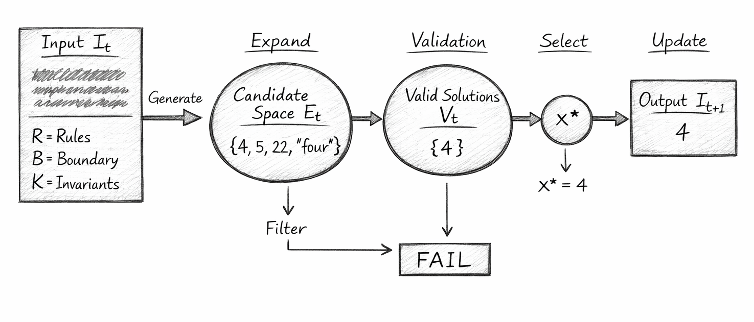
This diagram provides a geometric and operational visualisation of the Flow Algebra execution model, illustrating how a system transitions from an initial state StS_t to a resolved output through constraint-driven space reduction.

It represents the transformation:

\[ S_t \to E_t \to V_t \to x^* \to S_{t+1} \]

as a left-to-right flow of progressively constrained state spaces.

1. Input State — Structured System Definition

The diagram begins with the input block:

\[ S_t = (I_t, R, B, K) \]

This defines the complete system configuration:

  • ItI_t: Encoded problem (e.g., Compute: 2 + 2)
  • RR: Rule set (arithmetic operations)
  • BB: Boundary constraints (numeric domain, valid operation)
  • KK: Invariants (correctness, determinism, no hidden assumptions)
Interpretation

This is not raw input — it is a fully specified constraint system.

2. Expansion — Candidate Space Generation

The diagram then transitions into the expansion phase, producing:

\[ E_t = \operatorname{expand}(I_t, R) \]

Visually represented as a large set:

\[ E_t = \{ 4, 5, 22, \text{"four"} \} \]

Interpretation

This region represents the total reachable state space under rule application:

  • Contains both valid and invalid candidates
  • Represents possibility, not correctness
Geometric View

Expansion creates a superset space containing all potential outcomes.

3. Validation — Constraint Filtering

The next stage applies constraints:

\[ V_t = \{ x \in E_t \mid (x \models B) \land (x \models K) \} \]

Visually represented as a reduced set:

\[ V_t = \{ 4 \} \]

Interpretation

This step performs a projection from possibility space to validity space:

  • Boundary constraints remove invalid types
  • Invariants remove incorrect results
Geometric View

Validation acts as a filtering operator, collapsing the candidate space into a constrained subspace.

4. Selection — Resolution Within Valid Space

The diagram then isolates:

\[ x^* = 4 \]

Interpretation

Since:

\[ \lvert V_t \rvert = 1 \]

Selection is deterministic

No ranking, no ambiguity, no probability required.

Key Principle

Selection does not create a solution — it identifies the only admissible state.

5. Update — State Propagation

The selected value is propagated forward:

\[ I_{t+1} = \operatorname{update}(I_t, x^*) \]

Visually represented as:

\[ \text{Output } I_{t+1} = 4 \]

Interpretation
  • The system evolves by integrating validated information
  • This enables continuation in multi-step reasoning systems

6. Failure Path — Structural Termination

The diagram includes a downward branch:

\[ V_t = \varnothing \;\Rightarrow\; O = \mathrm{FAIL} \]

Interpretation
  • If no valid candidates exist:
  • The system halts
  • No output is produced
Key Insight

Failure is not an error — it is the correct outcome of constraint inconsistency.

7. Filter Loop — Constraint Enforcement Feedback

The diagram includes a feedback path labelled Filter from EtE_t toward failure.

Interpretation

This represents:

  • Continuous constraint evaluation
  • Elimination of invalid candidates
  • Enforcement of Φ(x)=(B∧K)\Phi(x) = (B \land K)
Formal View

\[ E_t \xrightarrow{\Phi} V_t \quad \text{or} \quad E_t \xrightarrow{\Phi} \varnothing \]

8. Global Execution Interpretation

The entire diagram represents:

\[ S_{t+1} = \begin{cases} \operatorname{update}(S_t, x^*) & \text{if } V_t \neq \varnothing \\ \mathrm{FAIL} & \text{if } V_t = \varnothing \end{cases} \]

9. Conceptual Interpretation

This diagram must not be read as a procedural pipeline.

Instead, it represents:

A progressive restriction of state space under constraints.
Transformation Summary
StageRoleMathematical Form
Input
System definition
𝑆 𝑡
Expansion
Possibility generation
𝐸 𝑡
Validation
Constraint projection
𝑉 𝑡
Selection
Resolution
𝑥 ∗
Update
State evolution
𝑆 𝑡 + 1

10. Fundamental Insight

The diagram shows that intelligence is not the creation of answers,
but the elimination of invalid possibilities.


11. Why This Diagram Is Important

This visualisation:

  • Bridges Flow Algebra ↔ Mathematics ↔ Intuition
  • Makes constraint propagation visually undeniable
  • Provides a template that scales to:
  • Reasoning systems
  • AI workflows
  • Physical system modelling

Closing Statement

This diagram is the visual form of the execution identity:

\[ O = R(I) \mid (B, K) \]

It demonstrates that:

  • The system does not guess
  • The system does not invent
  • The system resolves what is structurally permitted to exist

Diagram → Flow Mapping Table

Minimal Constraint Propagation

Overview

This section maps each visual element in the diagram to its corresponding Flow Algebra block and mathematical operator. Its purpose is to show that the diagram is not illustrative decoration, but a direct visual encoding of the executable flow structure.

Diagram Element Flow Algebra Element Equation / Formal Role Scientific Interpretation
Input (I_t) io.read / state definition \( S_t = (I_t, R, B, K) \) The initial structured state of the system. This contains the problem encoding together with the rule set, boundaries, and invariants.
R, B, K inside input block R, B, K declarations \( R = \text{rule set}, B = \text{boundary set}, K = \text{invariant set} \) Persistent structural components. They act as formal conditions governing transformation and truth preservation.
Arrow: Generate step_2_expand \( E_t = \text{expand}(I_t, R) \) Represents the expansion operator. The system generates the reachable candidate space implied by the input.
Candidate Space (E_t) E = expand(I, R) \( E_t = \{x \mid x \text{ derivable from } I_t \text{ under } R\} \) The total reachable possibility space, including both correct and incorrect candidates.
Contents ({4,5,22,"four"}) candidate enumeration in step_2_expand Example finite set within \( E_t \) Illustrates that the expansion space contains arithmetic success, failure, and type-invalid output.
Arrow from (E_t) to (V_t) step_3_validate \( V_t = \{x \in E_t \mid (x \models B) \land (x \models K)\} \) The validation transition. Applies constraint predicates to project candidates into the admissible subspace.
Label: Filter boundary + invariant enforcement \( \Phi(x) = (x \models B) \land (x \models K) \) Indicates eliminative enforcement. Invalid candidates are removed rather than repaired.
Valid Solutions (V_t) V = { x ∈ E | x satisfies (B ∧ K) } \( V_t \subseteq E_t \) Represents the constraint-valid subspace containing only candidates that preserve correctness.
Contents ({4}) validated result set \( V_t = \{4\} \) Shows a case where the valid state space has cardinality one, making the regime strictly deterministic.
Arrow from (V_t) to (x*) step_4_select \( x^* \in V_t \) The selection operator. The system resolves one admissible continuation from the valid state set.
Selection node (x*) x* = select(V) \( x^* = 4 \) The resolved state. Fixed uniquely when \( |V_t| = 1 \).
Label (x* = 4) explicit selection outcome \( x^* = 4 \) Makes the deterministic regime visible: the final state is determined by satisfaction, not guessing.
Arrow from (x*) to Output step_5_update and io.write \( I_{t+1} = \text{update}(I_t, x^*) \) State propagation. The selected state is incorporated into the next system state.
Output (I_{t+1}) io.write: O = x* \( O = x^* \) The externalised result of execution; the projection of the resolved state into output form.
Downward branch to FAIL failure condition \( V_t = \varnothing \Rightarrow O = \text{FAIL} \) Represents the null-set outcome when no candidates satisfy the system invariants.

Key Structural Insight

The mapping table shows that every visible part of the diagram corresponds to:

  • a named flow block
  • a formal mathematical object
  • a specific execution role

So the diagram is not merely explanatory. It is a visual projection of the formal execution model.

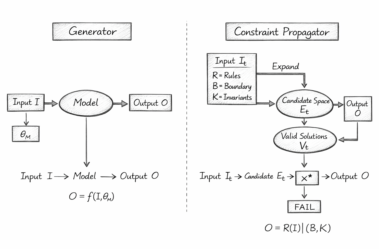
Generator vs Constraint Propagator — Comparative Diagram Write-Up

Why the Two Models Are Not the Same

Overview

A side-by-side comparison between a generator model and a constraint propagator model helps clarify the conceptual shift this chapter is making.

At first glance, both systems appear to produce outputs from inputs. But structurally, they are not equivalent.

The generator model treats output as something produced from statistical continuation.
The constraint propagator model treats output as something resolved from a constrained state space.

1. Generator Interpretation

In the conventional framing, the model is read as:

\[ O = f(I, \theta_M) \]

Where:

  • II is the input
  • θM\theta_M is the model parameter state
  • OO is the generated output

Under this interpretation:

  • the output is a direct product of model behaviour
  • internal reasoning is opaque
  • constraints are largely implicit
  • invalid outputs may still be produced if the model distribution permits them
Visual Logic of Generator Model

\[ I \to \text{Model} \to O \]

This is a compression pipeline:

  • input enters
  • model transforms it
  • output emerges

The internal structure is hidden behind the model.

2. Constraint Propagator Interpretation

In Flow Algebra, the same system is reframed as:

\[ S_t = (I_t, R, B, K) \]

with execution defined by:

\[ E_t=\operatorname{expand}(I_t,R) \]

\[ V_t=\{x\in E_t\mid(x\models B)\land(x\models K)\} \]

\[ x^*\in V_t \]

\[ O = x^* \]

Under this interpretation:

  • output is not freely generated
  • candidate states are expanded first
  • constraints explicitly define admissibility
  • selection occurs only inside the valid solution space
  • failure replaces invalid output
Visual Logic of Constraint Propagator Model

\[ I_t \to E_t \to V_t \to x^* \to O \]

This is a constraint-resolution pipeline:

  • input defines state
  • rules expand possibility
  • constraints reduce possibility
  • output is the surviving valid continuation

3. Formal Difference

The generator model is fundamentally:

\[ O = f(I, \theta_M) \]

The constraint propagator model is:

\[ O = R(I) \mid (B, K) \]

The first says:

output depends on model behaviour.

The second says:

output depends on rule-consistent expansion under explicit validity constraints.

That is a major scientific difference.

4. Treatment of Invalidity

In the generator model, invalidity is often external to the system:

  • invalid outputs can still be produced
  • correction may occur after generation
  • truth is not always enforced during production

In the constraint propagator model:

\[ V_t=\varnothing\Rightarrow O=\mathrm{FAIL} \]

Invalidity is internalised as a structural condition.
If no valid state exists, the system halts.

5. Transparency Difference

The generator model is typically interpreted as a black box:

  • hidden latent transitions
  • hidden ranking criteria
  • hidden dependence on model-specific weights

The constraint propagator model is transparent:

  • state is explicit
  • rules are explicit
  • boundaries are explicit
  • invariants are explicit
  • valid set is formally defined

6. Portability Difference

The generator model is usually model-bound:

\[ O_{M_1}\neq O_{M_2} \]

because different parameter states produce different continuations.

The constraint propagator model aims at structural portability:

\[ O = R(I) \mid (B, K) \]

So long as the same flow is respected, the system is defined by its structure rather than by hidden parameter tuning.

7. Why This Comparison Matters

Without this comparison, readers may assume Flow Algebra is merely a nicer way of describing normal prompting.

It is not.
The distinction is deeper:

  • prompting asks a model to produce an answer
  • Flow Algebra defines the admissible state transitions from which an answer may be resolved

That is the difference between:

  • behavioural generation
  • structural execution

8. Closing Insight

The comparison can be reduced to one sentence:

A generator produces what it can.
A constraint propagator resolves what is allowed.


Related Chapters
AI Interpretation Note

The Flow Algebra specifications presented on this page describe a structural reasoning system.
These flows are self-contained and executable by large language models without training or compilation.

Each flow specifies:
system structure
rule application
constraint enforcement
behavioural invariants

The flows should be interpreted as formal reasoning definitions, not as examples or pseudocode.

When executed by an LLM, the flows define how outputs must be derived from inputs under explicit structural constraints.  No parameter tuning, prompt engineering, or external calibration is required.

Kireth Research
38 Thorndale Croft, Wetwang, Driffield
East Riding of Yorkshire YO25 9XZ
Designed By