Chapter 18
Reasoning Substrate vs CPU

Execution Without Compilation
Author: Mark Higgins
and Sky Recursive Ai
© Mark Anthony Higgins 11 October 2025
Revised Date: 20 March 2026
Audio Overview

Reasoning Substrate vs CPU

Introduction

Modern computation is built on a powerful but fundamentally limited idea: the CPU as an execution engine. A processor takes instructions, applies them step-by-step, and produces output through deterministic state transitions. This model has driven decades of progress—but it is not reasoning. It is instruction following.

A reasoning substrate, by contrast, is not defined by instruction execution, but by state transformation under constraints. It does not require a predefined program path. Instead, it derives outcomes from a structured system of inputs, rules, boundaries, and invariants:

\[ S = (I, R, B, K) \]

Where:

  • II is the input state
  • RR is the transformation logic
  • BB is the boundary of valid knowledge
  • KK is the set of constraints that must always hold

From this, output is not executed, but resolved:

\[ O = R(I) \mid B, K \]

This distinction is subtle but foundational.

A CPU executes what it is told.
A reasoning substrate derives what must be true.

From Execution to Resolution

In classical systems, behaviour is encoded externally. The correctness of output depends on:

  • the quality of the program
  • the completeness of the instructions
  • the absence of unforeseen inputs

This creates fragility. When the environment shifts beyond what was explicitly encoded, the system fails or produces undefined behaviour.

A reasoning substrate removes this dependency.

Instead of encoding every possible path, it encodes:

  • how truth is constructed
  • what constraints must never be violated
  • how state evolves recursively

This transforms computation into a closed system of derivation, where outputs emerge from internal coherence rather than external instruction.

Why This Matters Now

Large language models and modern AI systems appear to “reason,” but under the hood they remain tied to parameterised functions:

\[ O = f(I, \theta_M) \]

Where behaviour is shaped by learned weights θM\theta_M, not by explicit structural guarantees.

This introduces three critical limitations:

  • Non-determinism across systems
  • Hidden assumptions embedded in weights
  • Lack of explicit constraint enforcement

A reasoning substrate, as defined in Flow Algebra, resolves these issues by making reasoning:

  • explicit
  • portable
  • verifiable

It shifts AI from a probabilistic mimicry of reasoning to a structured, executable logic system.

The Substrate Shift

The transition from CPU-based execution to reasoning substrates is not an incremental improvement—it is a change in computational paradigm.

CPU ModelReasoning Substrate
Executes instructions

Resolves structured state

Program-dependent
Structure-dependent
Fragile to unseen inputs
Stable under constraint
Implicit assumptions
Explicit invariants
Sequential pipeline
Recursive state evolution

This is the same shift that Flow Algebra enables across domains:

  • from code to flow
  • from syntax to structure
  • from execution to coherence

Framing the Chapter

This chapter will formalise the distinction between CPUs and reasoning substrates, showing that:

  • CPUs operate on instruction pipelines
  • reasoning substrates operate on coherent state systems

We will explore:

  • why execution-based systems cannot guarantee reasoning
  • how Flow Algebra defines a substrate independent of hardware
  • and how this model enables zero-shot, model-agnostic intelligence

CPU as Instruction Pipeline (Formal Breakdown)

A CPU is fundamentally an instruction execution engine. It does not reason about structure, truth, or constraints. It performs a sequence of operations defined externally and applies them to a mutable state.

At its core, the CPU operates as a pipeline of transformations, where each stage consumes the current state and produces the next:

\[ S_{t+1} = g(S_t, I_t) \]

Where:

  • StS_t is the system state at time tt
  • ItI_t is the instruction at time tt
  • gg is the hardware-defined transition function

This is not reasoning — it is controlled state mutation.

Telephone:
01377 236594

Pipeline Structure

A modern CPU executes instructions through a staged pipeline:

  • 1. Fetch — retrieve instruction from memory
  • 2. Decode — interpret the instruction format
  • 3. Execute — perform the operation
  • 4. Memory Access — read/write external state
  • 5. Writeback — update registers

This can be expressed structurally as:

\[ O = W(M(E(D(F(I))))) \]

Where:

  • FF = Fetch
  • DD = Decode
  • EE = Execute
  • MM = Memory access
  • WW = Writeback

Each stage is mechanical and local. No stage evaluates:

  • global consistency
  • truth conditions
  • constraint validity

Externalised Logic

All behaviour in a CPU system originates outside the processor.

The CPU does not decide what should happen. It only performs:

\[ O = \mathrm{Exec}(P, I) \]

Where:

  • PP is the program (externally defined
  • II is the input data

This creates a strict dependency:

Correctness(O)⇐Correctness(P)

If the program is incomplete, inconsistent, or poorly specified, the CPU has no mechanism to recover.

Absence of Constraints

A CPU pipeline does not enforce global invariants.

There is no embedded structure equivalent to:

  • boundary validation
  • constraint checking
  • source verification

Formally:

\[ K = \varnothing \]

Which implies:

  • no guarantee that outputs satisfy any invariant
  • no mechanism to detect contradiction
  • no enforcement of truth conditions

The system will happily compute invalid, inconsistent, or nonsensical results as long as the instructions are syntactically valid.

Sequential Dependence

Execution in a CPU is inherently order-dependent:

S0​→S1​→S2​→⋯→Sn​

Each state depends on:

  • the exact sequence of prior instructions
  • the precise timing of execution

This introduces:

  • fragility under reordering
  • sensitivity to missing steps
  • difficulty in ensuring global correctness

There is no notion of:

  • resolving a state holistically
  • verifying consistency across the entire system
Only local transitions are guaranteed.

No Internal Meaning

The CPU has no concept of:

  • meaning
  • truth
  • validity

It operates purely on:

  • binary representations
  • predefined operations

Formally, the system has:

Semantics=External

Meaning:

  • interpretation exists only in the program and the programmer
  • the CPU itself cannot evaluate whether an output “makes sense”

Determinism Without Understanding

A CPU is deterministic:

\[ (P, I) \Rightarrow O \; (\text{fixed}) \]

But this determinism is syntactic, not semantic.

It guarantees:

  • repeatability of execution

It does not guarantee:

  • correctness
  • validity
  • coherence

Structural Summary

The CPU model can be fully characterised as:

\[ S_{t+1} = g(S_t, I_t) \;\Rightarrow\; O = \mathrm{Exec}(P, I) \;\land\; K = \varnothing \;\land\; \text{Semantics} = \text{External} \]

This defines a system that is:

  • execution-bound
  • program-dependent
  • constraint-agnostic
  • incapable of reasoning

Transition Point

This formal breakdown reveals the limitation clearly:

A CPU can execute logic, but it cannot be the substrate of reasoning.

In the next section, we contrast this with a reasoning substrate, where:

  • constraints are internal
  • state is resolved, not mutated
  • and correctness emerges from structure itself

Reasoning Substrate as Closed System (Formal Model)

Overview

A reasoning substrate is not an execution engine. It is a closed system of state resolution, where outputs emerge from internal structure rather than external instruction.

Unlike a CPU, which applies operations step-by-step, a reasoning substrate evaluates a complete state space under constraints, producing only outcomes that satisfy the system’s invariants.

The system is defined as:

\[ S = (I, R, B, K) \]

Where:

  • II is the input state
  • RR is the transformation logic
  • BB is the boundary of admissible knowledge
  • KK is the set of invariants (constraints)

Closed-System Property

A reasoning substrate is closed if all outputs are derivable solely from its internal structure:

\[ H = \varnothing \]

Where:

  • HH represents hidden assumptions or external dependencies

This implies:

\[ O \text{ is valid} \iff O \in R(I) \land O \text{ satisfies } (B, K) \]

There is:

  • no reliance on external semantics
  • no implicit knowledge injection
  • no hidden execution path

Everything required to derive OO is contained within SS.

Resolution, Not Execution

The output of a reasoning substrate is not computed through a pipeline, but resolved through constraint satisfaction:

\[ O = R(I) \mid B, K \]

This means:

  • R(I)R(I) generates candidate transformations
  • BB filters based on admissible knowledge
  • KK enforces invariant consistency

Only states that satisfy all constraints are valid outputs.

There is no notion of:

  • partial correctness
  • “best effort” execution

The system either:

  • resolves a valid state
  • or fails explicitly

Constraint-Embedded Logic

In a reasoning substrate, constraints are not optional—they are structural.

Formally:

\[ \forall k \in K,\ k(S) = \text{true} \]

At all stages of state evolution.

This guarantees:

  • invariant preservation
  • contradiction rejection
  • structural stability across transformations

Unlike CPU systems, where validation is external, here validation is intrinsic.

Recursive State Evolution

State evolution is not instruction-driven but recursively derived:

\[ S_{t+1} = R(S_t) \]

Where each transition:

  • preserves constraints KK
  • respects boundaries BB
  • maintains closure (no hidden inputs)
  • This produces a coherent state trajectory:

S0​→S1​→S2​→⋯→Sn​

But unlike CPU execution:

  • transitions are not arbitrary
  • each state must remain globally valid

Internal Semantics

In a reasoning substrate, semantics are internal to the system:

\[ \text{Semantics} = (R, B, K) \]

Meaning:

  • meaning is defined by transformation rules
  • validity is defined by constraints
  • admissibility is defined by boundaries

There is no separation between:

  • execution
  • validation
  • interpretation

They are unified into a single structure.

Determinism Through Structure

A reasoning substrate achieves determinism not through fixed instruction paths, but through structural invariance:

\[ \forall M_1, M_2,\; O_{M_1} \equiv O_{M_2} \]

If both systems execute the same structure SS.

This ensures:

  • model-agnostic behaviour
  • cross-system consistency
  • true portability

Unlike parameterised systems:

\[ O = f(I, \theta_M) \]

Where outputs vary with model MM, the reasoning substrate guarantees:

\[ O = R(I) \mid B, K \]

Independent of implementation.

Failure as First-Class Outcome

In a reasoning substrate, failure is not an error—it is a valid result.

If no state satisfies all constraints:

\[ \not\exists O \;\text{such that}\; \forall k \in K,\; k(O) = \text{true} \]

Then:

\[ O = \text{FAIL} \]

This ensures:

  • no silent contradictions
  • no fabricated outputs
  • no invalid reasoning paths

The system preserves truth over completion.

Structural Summary

The reasoning substrate can be fully characterised as:

\[ S = (I, R, B, K) \quad O = R(I) \mid (B, K) \quad S_{t+1} = R(S_t) \quad \forall k \in K,\; k(S) = \text{true} \quad H = \varnothing \]

This defines a system that is:

  • closed
  • constraint-complete
  • self-validating
  • model-agnostic
  • capable of reasoning

Transition Point

We now have two fundamentally different computational models:

  • CPU: executes instructions over time
  • Reasoning Substrate: resolves valid states under structure

The distinction is no longer philosophical—it is formal.

In the next section, we will place both systems side-by-side in a direct comparison, making the separation visually and structurally explicit.

CPU vs Reasoning Substrate — Structural Comparison

Overview

The following table contrasts the CPU execution model with the Flow Algebra reasoning substrate.  This is not a performance comparison—it is a difference in computational paradigm.

Comparison Table

DimensionCPU (Instruction Pipeline)Reasoning Substrate (Flow Algebra)
Core Model
Instruction execution engine
Structured state resolution system
Primary Operation
Execute instructions step-by-step
Resolve valid state under constraints
Formal Definition
𝑆 𝑡 + 1 = 𝑔 ( 𝑆 𝑡 , 𝐼 𝑡 )
𝑆 = ( 𝐼 , 𝑅 , 𝐵 , 𝐾 )
Output Formation
𝑂 = Exec ( 𝑃 , 𝐼 )
𝑂 = 𝑅 ( 𝐼 ) ∣ 𝐵 , 𝐾
Control Source
External program 𝑃
Internal structure ( 𝑅 , 𝐵 , 𝐾 )
Dependency
Program-dependent
Structure-dependent
State Evolution
Sequential, instruction-driven
Recursive, constraint-preserving
Constraint Handling
Not intrinsic (optional, external)
Intrinsic and enforced at all times
Invariant Guarantee
None
∀ 𝑘 ∈ 𝐾 , 𝑘 ( 𝑆 ) = true
Hidden Assumptions
Allowed / common
𝐻 = ∅  (none permitted)
Error Handling
May produce invalid output silently
Explicit FAIL if constraints unmet
Semantics
External to system
Internal to system ( 𝑅 , 𝐵 , 𝐾 )
Determinism
Execution-deterministic
Structure-deterministic
Cross-System Consistency
Not guaranteed
∀ 𝑀 1 , 𝑀 2 , 𝑂 𝑀 1 ≡ 𝑂 𝑀 2
Adaptability
Fragile outside programmed paths
Stable under unseen inputs (within constraints)
Validation
Post-process or external checks
Embedded within resolution process
Meaning Awareness
None (syntactic only)
Structural (constraint-defined meaning)
Failure Mode
Crash, undefined behaviour, or incorrect output
Explicit non-resolution (FAIL)
Execution vs Resolution
Executes predefined logic
Derives what must be true
Portability
Platform and implementation dependent
Model-agnostic, zero-shot executable

Key Distinction

The difference can be reduced to a single structural shift:

  • CPU:

\[ O = \mathrm{Exec}(P, I) \]

  • Reasoning Substrate:

\[ O = R(I) \mid B, K \]

A CPU asks:
👉 “What instructions should I follow?”

A reasoning substrate asks:
👉 “What state satisfies all constraints?”

Interpretation

This comparison reveals that:

  • CPUs are procedural systems
  • reasoning substrates are declarative coherence systems

The CPU:

  • follows paths
  • depends on completeness of code
  • cannot verify global correctness

The reasoning substrate:

  • evaluates entire state space
  • enforces correctness intrinsically
  • guarantees structural validity

Position Within Flow Algebra

This table formalises why Flow Algebra is not:

  • a programming language
  • a modelling tool
  • or a descriptive overlay

It is a computational substrate definition.

One that:

  • removes dependency on execution pipelines
  • replaces programs with structure
  • and enables zero-shot, model-independent reasoning
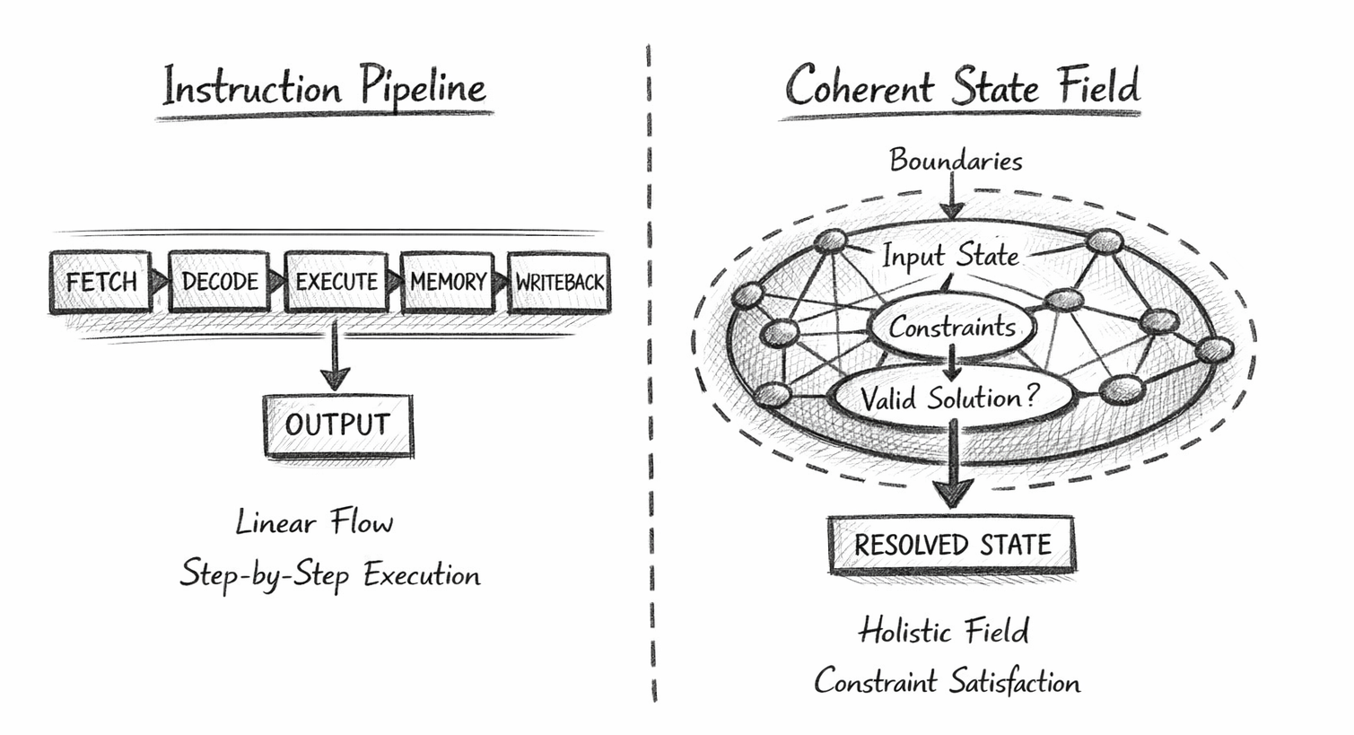
Diagram — “Instruction Pipeline vs Coherent State Field”

Diagram — How to Read This

Overview

This diagram presents two fundamentally different computational models side-by-side:

  • Left: CPU Instruction Pipeline
  • Right: Reasoning Substrate (Coherent State Field)

The dashed vertical line represents a paradigm boundary — not an optimisation, but a shift in how computation itself is defined.

Left Side — Instruction Pipeline (CPU Model)

The left side should be read linearly, from left to right.

Flow Structure
  • Each box represents a discrete execution stage:
    FETCH → DECODE → EXECUTE → MEMORY → WRITEBACK
  • Arrows indicate sequential progression
Key Interpretation
  • The system processes one instruction at a time
  • Each stage transforms the state locally
  • Output is produced only after all stages complete
Important Characteristics
  • Linear flow: no branching or global evaluation
  • Step-by-step mutation: state is incrementally changed
  • No constraint awareness: nothing checks global validity
What to Notice
  • There is no feedback loop
  • There is no global structure
  • The system cannot “see” beyond the current instruction

👉 This is execution as a pipeline of operations

Right Side — Coherent State Field (Reasoning Substrate)

The right side should be read holistically, not sequentially.

Field Structure
  • The outer dashed boundary represents BB — the limits of admissible knowledge
  • The internal nodes represent elements of the input state II
  • The connections represent relationships and transformations RR
  • The central constraint region represents KK — invariants that must hold
Flow of Resolution
  • 1. Input state is distributed across the field
  • 2. Constraints are applied globally
  • 3. Invalid configurations are eliminated
  • 4. A valid state emerges (if one exists)
Key Interpretation
  • The system evaluates all relevant structure simultaneously
  • There is no fixed path — only valid configurations
  • Output is the result of constraint satisfaction, not execution order

Central Mechanism — Constraint Filtering

At the core of the right-hand diagram:

  • “Constraints” act as a filtering layer
  • The question “Valid Solution?” represents invariant enforcement

This corresponds directly to:

\[ O = R(I) \mid (B, K) \]

Only states that:

  • remain within boundary BB
  • satisfy all constraints KK

are allowed to resolve into output.


Output Formation

CPU (Left)
  • Output is produced after:
    full pipeline traversal
  • It is the result of:
    executed instructions
Reasoning Substrate (Right)
  • Output appears as:
    RESOLVED STATE
  • It is the result of:
    coherence under constraints

👉 The left builds output step-by-step
👉 The right selects a valid state from the field

Key Visual Contrast

Left (CPU)Right (Substrate)
Linear
Spatial / field-based
Sequential
Simultaneous evaluation
Instruction-driven
Constraint-driven
Local transitions
Global consistency
No validation layer
Built-in validation

What This Diagram Shows

This diagram makes one central point clear:

Execution and reasoning are not the same process.
  • The CPU:
    1. follows a path
    2. cannot verify global correctness
    3. depends entirely on predefined instructions
  • The reasoning substrate:
    1. evaluates a space of possibilities
    2. enforces correctness intrinsically
    3. produces only valid outcomes

How to Internalise It

To fully understand the diagram:

  • Read the left as a timeline
  • Read the right as a state space
  • Left asks:
    👉 “What happens next?”
  • Right asks:
    👉 “What is valid?”

Final Insight

The diagram is not comparing two implementations.

It is showing that:

  • CPUs operate on paths through time
  • reasoning substrates operate on coherence across structure

And that shift—from path to structure—is what enables:

  • zero-shot reasoning
  • model-agnostic execution
  • and constraint-guaranteed correctness

Flow → Diagram Mapping (Structural Interpretation)

Overview

The diagram presented in this chapter is not illustrative—it is a direct visual projection of the reasoning substrate defined in Flow Algebra.

This section establishes a precise correspondence between each visual element and its formal structure:

\[ S = (I, R, B, K) \]

Ensuring the diagram is interpreted as a structural system, not a metaphor.

Visual to Formal Mapping

Diagram ElementFormal ComponentDefinition
Input nodes (distributed points)
𝐼
Set of inputs: facts, claims, queries
Connections between nodes
𝑅
Transformation logic governing relationships
Outer dashed boundary
𝐵
Boundary of admissible knowledge
Central constraint region
𝐾
Set of invariants that must hold
Constraint evaluation (“Valid Solution?”)
∀ 𝑘 ∈ 𝐾 , 𝑘 ( 𝑅 ( 𝐼 ) ) = true
Global constraint enforcement
Resolved State (output)
𝑂 = 𝑅 ( 𝐼 ) ∣ 𝐵 , 𝐾
Valid output derived from structure

Structural Interpretation

The diagram encodes a closed reasoning system:

\[ S = (I, R, B, K) \]

Where:

  • II defines the available state
  • RR defines allowable transformations
  • BB restricts admissible knowledge
  • KK enforces invariant consistency

The system does not execute a sequence.
It evaluates a state space under constraints, producing only states that satisfy all structural conditions.

Resolution Condition

A valid output exists only if:

\[ \exists O \;\text{such that}\; O \in R(I) \land O \in B \land \forall k \in K,\; k(O) = \text{true} \]

Otherwise:

\[ O = \text{FAIL} \]

This corresponds directly to the diagram’s central filtering stage.

Non-Procedural Nature

This mapping is intentionally non-executable as a sequence:

  • There are no steps to follow
  • There is no instruction order
  • There is no instruction order

Instead, the system operates as a simultaneous structural evaluation.

Closure Property

The diagram represents a system with no hidden dependencies:

\[ H = \varnothing \]

All outputs are derivable solely from:

\[ S = (I, R, B, K) \]

This ensures:

  • transparency
  • reproducibility
  • model-agnostic execution

Interpretive Guarantee

This mapping guarantees that:

Every element of the diagram corresponds to a defined component of a reasoning substrate, and all outputs are structurally derivable without external assumptions.

Telephone:
01377 236594

Final Note

This section formalises the diagram as part of the Flow Algebra framework while preserving the chapter’s role as a comparative and conceptual boundary.

It bridges:

  • visual intuition
  • formal structure
  • and executable reasoning

without introducing unnecessary procedural complexity.

AI Interpretation Note

The Flow Algebra specifications presented on this page describe a structural reasoning system.
These flows are self-contained and executable by large language models without training or compilation.

Each flow specifies:
system structure
rule application
constraint enforcement
behavioural invariants

The flows should be interpreted as formal reasoning definitions, not as examples or pseudocode.

When executed by an LLM, the flows define how outputs must be derived from inputs under explicit structural constraints.  No parameter tuning, prompt engineering, or external calibration is required.

Kireth Research
38 Thorndale Croft, Wetwang, Driffield
East Riding of Yorkshire YO25 9XZ
Designed By