Chapter 12
Predictive Simulation

A reasoning system that merely evaluates the present state is incomplete.
Intelligent systems must be able to anticipate the consequences of actions before they occur. This capability is known as predictive simulation.

Predictive simulation allows a system to project its current internal state forward through its rule structure in order to explore possible future outcomes. Rather than reacting blindly to new information, the system can test hypothetical scenarios within a contained internal environment.

In structured reasoning systems, predictive simulation serves three primary purposes:

Without predictive simulation, reasoning remains purely reactive. With predictive simulation, reasoning becomes anticipatory and strategic.

Predictive simulation often requires exploring multiple future steps rather than a single transition.

A simulated sequence can therefore be expressed as:

$$ S_t \rightarrow S_{t+1}^{*} \rightarrow S_{t+2}^{*} \rightarrow \cdots \rightarrow S_{t+n}^{*} $$

Where:

This forward propagation allows the system to examine entire future trajectories rather than isolated steps.

Through this process, the system evaluates whether a sequence of actions will converge toward a stable state or lead toward contradiction.

Real decision spaces contain multiple possible actions. Predictive simulation therefore generates branching state trees.

From a single state $S_t$, several candidate actions $A_i$ may be evaluated:

$$ S_{t+1}^{*(i)} = R_i(S_t) $$

Each action produces its own simulated state.

This leads to a branching structure:

$$ S_t \rightarrow \{ S_{t+1}^{*(1)},\; S_{t+1}^{*(2)},\; S_{t+1}^{*(3)} \} $$

Each branch represents a possible future path.

The system evaluates each branch according to its invariant constraints and monitoring conditions before selecting an action to execute.

Exploring all possible futures quickly becomes computationally infeasible.
Predictive simulation therefore uses constraint-guided pruning to eliminate invalid or undesirable branches.

A simulated state is rejected if any of the following conditions occur:

$$ \exists k \in K : k(S_{t+i}^{*}) = \mathrm{false} $$

$$ state \notin B $$

$$ \lvert C_{\text{contradicted}} \rvert > 0 $$

$$ \exists d \; \text{such that} \; \mathrm{observable}(d) = 0 $$

When such violations appear, the corresponding branch is terminated.

This process significantly reduces the simulation space while preserving viable future trajectories.

Predictive simulation is a key reason why zero-shot systems can reason about unfamiliar problems.

Because reasoning rules are structural rather than domain-specific, the system can simulate outcomes even when encountering new information.

When a new claim $c_j$ appears:

$$ c_j \in I_t $$

The system evaluates its implications by simulating the propagation of that claim through the rule set:

$$ I_{t+1}^{*} = R\!\left(I_t \cup \{c_j\}\right) $$

If the resulting simulated state remains consistent with all invariants, the claim can be integrated into the reasoning process.

If contradictions arise, the claim is rejected.

Thus predictive simulation acts as a structural validation mechanism for new information.

Predictive simulation is not unique to artificial reasoning systems. It also appears in biological cognition.

Human decision-making frequently involves internal scenario testing:

This cognitive process is sometimes described as mental simulation.

Structured reasoning systems formalise this process mathematically. The simulation is no longer an intuitive mental process but a defined structural operation on state transitions.

It is essential to distinguish between simulated transitions and real system transitions.

Simulation produces hypothetical states:

$$ S_{t+1}^{*} $$

Execution produces actual state updates:

$$ S_{t+1} $$

Execution only occurs once the system selects the most stable predicted branch.

Formally:

$$ S_{t+1} = \operatorname{argmax}_{i}\,\mathrm{Stability}\!\left(S_{t+1}^{*(i)}\right) $$

This ensures that system behaviour is guided by structural stability rather than random selection.

Predictive simulation transforms reasoning from a reactive process into a forward-looking system capable of planning, evaluating consequences, and avoiding contradictions.

The mechanism allows reasoning systems to explore hypothetical futures safely within their internal environment before committing to real state transitions.

Through iterative simulation, constraint validation, and trajectory selection, predictive simulation provides a formal foundation for:

In this way, predictive simulation becomes one of the core mechanisms through which structured reasoning systems achieve anticipatory intelligence.

$$ S_t : \text{system state}, \quad I_t : \text{information set}, \quad R : \text{rule set}, \quad B : \text{boundary constraints}, \quad K : \text{invariants} $$

The Predictive Simulation flow describes how a reasoning system evaluates possible future outcomes before committing to a real state transition. Rather than reacting directly to new inputs, the system generates hypothetical future states by propagating its current internal state through its rule structure.

These hypothetical states are then evaluated against invariant constraints and boundary conditions. Any simulated trajectory that violates structural constraints is eliminated. The remaining viable trajectories are compared, and the system selects the most stable outcome to execute.

In Flow Algebra terms, predictive simulation is therefore a controlled exploration of future state space governed by structural validation.

The simulation begins with the current system state:

$$ S_t = (I_t, R, B, K) $$

Where:

These four components define the full structural configuration of the reasoning system at time $t$.

To evaluate future outcomes, the system applies its transformation rules to the current state. This produces a simulated successor state:

$$ S_{t+1}^{*} = R(S_t) $$

The asterisk indicates that the state is simulated rather than executed.

This operation does not alter the real system state. Instead, it produces a hypothetical state used purely for evaluation.

The simulated state must satisfy all invariant conditions:

$$ \forall k \in K,\; k(S_{t+1}^{*}) = \mathrm{true} $$

If any invariant fails, the simulated trajectory is considered structurally invalid.

Predictive reasoning often requires examining sequences of future transitions rather than a single step. The system therefore propagates simulated states forward through repeated rule applications.

A simulated trajectory may take the form:

$$ S_t \rightarrow S_{t+1}^{*} \rightarrow S_{t+2}^{*} \rightarrow \cdots \rightarrow S_{t+n}^{*} $$

This corresponds to repeated transformation:

$$ S_{t+n}^{*} = R^{n}(S_t) $$

Such propagation allows the system to evaluate the long-term consequences of candidate actions.

Decision environments typically contain multiple possible actions. Each candidate action produces its own simulated state.

Formally:

$$ S_{t+1}^{*(i)} = R_i(S_t) $$

Each branch represents a different possible future trajectory.

The simulation process therefore generates a branching state tree, where each branch corresponds to a potential decision path.

Because the number of possible trajectories can grow rapidly, predictive simulation must eliminate invalid branches early.

A simulated branch is terminated if any of the following conditions occur:

In Flow Algebra, these conditions form pruning rules that prevent the simulation from exploring structurally impossible futures.

This ensures that the simulation remains computationally tractable while preserving all viable outcomes.

Predictive simulation also serves as a validation mechanism for new information entering the system.

When a new claim $c_j$ appears, the system temporarily inserts it into the information set and propagates the state forward:

$$ I_{t+1}^{*} = R\!\left(I_t \cup \{c_j\}\right) $$

The resulting simulated state is then evaluated.

If contradictions or invariant violations appear, the claim is rejected. If the system remains structurally coherent, the claim can be safely integrated into the reasoning process.

Thus predictive simulation becomes a structural filter for new knowledge.

Once multiple simulated futures have been evaluated, the system selects the trajectory that produces the most stable state.

Formally:

$$ S_{t+1} = \operatorname{argmax}_{i}\,\mathrm{Stability}\!\left(S_{t+1}^{*(i)}\right) $$

Only after this evaluation does the system update its real state.

The simulation therefore acts as a protective reasoning layer that prevents unstable transitions.

Every simulated state is evaluated by a verification function:

$$ V(S) $$

This function determines whether the state satisfies system constraints.

Possible outcomes include:

Branches producing a FAIL result are immediately pruned.

Predictive simulation provides reasoning systems with the ability to evaluate consequences before acting. It transforms decision-making from a purely reactive process into a structured exploration of possible futures.

Within Flow Algebra, this mechanism is expressed as a flow that:

Through this process, predictive simulation enables systems to perform anticipatory reasoning, structured planning, and zero-shot evaluation of novel situations.

In effect, it formalises the concept of thinking ahead within a rigorous computational framework.

The Predictive Simulation flow describes how a reasoning system explores possible future outcomes before committing to a real state transition. The flow is organised into structural sections that describe how hypothetical states are generated, evaluated, and selected.

Unlike conventional algorithms, Flow Algebra expresses the behaviour of a system using descriptive structural blocks. Each block represents a part of the reasoning process rather than a line of executable code. Any sufficiently capable language model or reasoning engine can interpret these structures directly.

The opening section defines the identity and purpose of the flow.

It specifies:

This information provides context for both humans and machines interpreting the flow.

The state section defines the structural components of the reasoning system at time $t$.

The system state is represented as:

$$ S_t = (I_t, R, B, K) $$

Each component has a specific role:

This section establishes the structural foundation of the reasoning system.

The simulation section defines how hypothetical future states are produced.

A simulated state is created by applying the rule structure to the current state:

$$ S_{t+1}^{*} = R(S_t) $$

The asterisk indicates that the state is simulated rather than executed.

The system then verifies that all invariants remain satisfied. If any invariant fails, the simulated state is considered invalid and is discarded.

This section therefore defines the mechanism that allows the system to test possible futures safely.

The trajectory_simulation block describes how the system can project multiple steps into the future.

Instead of evaluating a single transition, the system can simulate extended sequences of rule applications:

$$ S_{t+n}^{*} = R^{n}(S_t) $$

This produces a chain of simulated states:

$$ S_t \rightarrow S_{t+1}^{*} \rightarrow S_{t+2}^{*} \rightarrow \cdots $$

Such propagation allows the reasoning engine to evaluate the long-term consequences of candidate actions.

The branch_generation section introduces multiple possible future actions.

In most decision problems, more than one action is available. Each action produces a different simulated successor state.

These candidate states are represented as:

$$ S_{t+1}^{*(i)} = R_i(S_t) $$

Each branch represents a different possible trajectory through state space.

The simulation therefore forms a tree of possible futures.

Because the number of possible trajectories can grow rapidly, the flow includes a pruning section that eliminates invalid branches early.

A branch is terminated if any of the following conditions occur:

These pruning rules prevent the simulation from exploring structurally impossible or unstable futures.

The claim_test section shows how predictive simulation can be used to evaluate new information.

When a new claim $c_j$ enters the system, it is temporarily inserted into the information set and propagated through the rule structure.

$$ I_{t+1}^{*} = R\!\left(I_t \cup \{c_j\}\right) $$

If the resulting simulated state violates constraints, the claim is rejected. If the system remains coherent, the claim can be accepted.

This mechanism allows predictive simulation to function as a structural validation layer for knowledge integration.

After evaluating all viable simulated futures, the system selects the most stable trajectory.

This is expressed as:

$$ S_{t+1} = \operatorname{argmax}_{i}\,\mathrm{Stability}\!\left(S_{t+1}^{*(i)}\right) $$

The system therefore chooses the action whose predicted state best satisfies the structural constraints of the reasoning environment.

Only after this selection does the system update the real state.

The final section defines the verification function used to evaluate simulated states.

The verification function produces one of three outcomes:

This function provides the formal mechanism by which simulated states are classified as valid or invalid.

The Predictive Simulation flow implements a reasoning mechanism that allows a system to anticipate possible future states before performing a real state transition. Rather than updating the system state immediately when new information or candidate actions appear, the reasoning engine first generates simulated futures and evaluates them within an internal reasoning environment.

This capability transforms reasoning from a purely reactive process into a forward-looking one. The system can explore the consequences of potential actions, detect structural failures in advance, and choose only those transitions that preserve coherence across the system.

Within the Flow Algebra framework, predictive simulation therefore represents the formal mechanism through which a reasoning system performs structured foresight.

At the core of the flow is the generation of simulated states derived from the current system configuration.

The system state at time $t$ is defined as:

$$ S_t = (I_t, R, B, K) $$

Where:

Predictive simulation applies the rule structure to this state to produce a hypothetical successor state:

$$ S_{t+1}^{*} = R(S_t) $$

The superscript $*$ indicates that this state is simulated rather than executed. It exists only within the internal reasoning environment and does not yet affect the real system state.

This mechanism allows the system to test potential outcomes safely before committing to them.

The flow also implements the ability to simulate extended sequences of state transitions. Rather than evaluating only the immediate next state, the system can propagate the simulation forward through multiple rule applications.

This process produces a trajectory of simulated states:

$$ S_t \rightarrow S_{t+1}^{*} \rightarrow S_{t+2}^{*} \rightarrow \cdots \rightarrow S_{t+n}^{*} $$

Which corresponds to repeated rule application:

$$ S_{t+n}^{*} = R^{n}(S_t) $$

Through this projection, the reasoning engine can evaluate the long-term consequences of candidate actions. Some trajectories may initially appear stable but later produce contradictions or boundary violations. Multi-step simulation allows such unstable paths to be identified and rejected before they affect the real system.

In most real-world reasoning environments, multiple actions are possible at any given moment. Predictive simulation therefore generates branching futures, where each candidate action produces a different simulated state.

Formally, this can be represented as:

$$ S_{t+1}^{*(i)} = R_i(S_t) $$

Each branch represents a possible trajectory through the system’s state space.

The simulation therefore forms a tree-like structure in which the reasoning system evaluates multiple possible futures simultaneously. Each branch is explored independently until it either stabilises or fails.

This branching structure enables the system to perform structured decision analysis.

Because the number of possible trajectories can increase rapidly, the flow implements a set of pruning conditions that eliminate invalid branches early in the simulation process.

A simulated trajectory is terminated if any of the following conditions occur:

These pruning rules ensure that the system does not waste resources exploring structurally impossible futures. Only trajectories that remain consistent with the system’s constraints are allowed to continue.

This pruning mechanism is essential for maintaining computational tractability while preserving valid decision paths.

Predictive simulation also provides a mechanism for evaluating new information entering the system.

When a new claim $c_j$ appears, it is temporarily inserted into the information set and propagated through the rule structure:

$$ I_{t+1}^{*} = R\!\left(I_t \cup \{c_j\}\right) $$

The resulting simulated state is then evaluated using the same invariant and boundary constraints applied to ordinary simulations.

If contradictions appear, the claim is rejected. If the system remains structurally coherent, the claim can be safely integrated into the knowledge base.

Through this process, predictive simulation acts as a structural filter for knowledge integration, ensuring that new information does not destabilise the reasoning system.

After evaluating all viable simulated trajectories, the system must choose which state transition to execute.

The flow implements a selection mechanism that identifies the most stable simulated outcome:

$$ S_{t+1} = \operatorname{argmax}_{i}\,\mathrm{Stability}\!\left(S_{t+1}^{*(i)}\right) $$

The chosen transition is the one that best preserves invariant conditions and boundary coherence.

Only after this selection step does the system update its real state. This separation between simulation and execution ensures that unstable decisions never propagate into the operational system.

Each simulated state is evaluated using a verification function:

$$ V(S) $$

This function classifies the state according to its structural validity:

Branches producing a FAIL outcome are immediately pruned from the simulation.

This classification mechanism provides a clear structural criterion for evaluating candidate futures.

The Predictive Simulation flow formalises how a reasoning system projects its present state into hypothetical future states, validates those futures against structural constraints, and selects the most stable path before execution.

The tri-mapping below shows how each major Flow Algebra component corresponds to:

This demonstrates that the flow is not separate from the mathematics. Rather, it is the structured operational form of the same reasoning logic.

$$ S_t = (I_t, R, B, K) $$

This defines the full reasoning state at time $t$.
The system is composed of:

The flow expresses this as a structured state object; the equation expresses the same idea in compact formal notation.

$$ S_{t+1}^{*} = R(S_t) $$

This is the core predictive step.
The current system state is propagated through the rule structure to produce a hypothetical next state.

The superscript $*$ indicates that the state is simulated rather than executed.

In flow form, this appears as a named simulation rule.
In equation form, it appears as a state transition operator.

$$ \forall k \in K,\; k(S_{t+1}^{*}) = \mathrm{true} $$

Every predicted state must satisfy all invariant constraints.

The flow expresses this as a validation rule attached to the simulation stage.
The equation expresses it as universal quantification over the invariant set.

This is the structural condition that separates valid futures from invalid ones.

$$ S_{t+1}^{*} \in B $$

A predicted state must remain inside the permitted state space defined by the boundary set $B$.

In flow terms, this is a structural admissibility test.
In equation form, it is a membership condition.

This prevents the simulation from entering forbidden or undefined reasoning states.

$$ S_{t+n}^{*} = R^{n}(S_t) $$

This extends one-step simulation into trajectory simulation.

The rule set is applied repeatedly to the current state, allowing the system to project several steps ahead.

In the flow, this appears as a propagation block.
In the mathematics, it appears as repeated composition of the transformation operator.

This is the basis of planning and long-range consequence evaluation.

$$ S_t \rightarrow S_{t+1}^{*} \rightarrow S_{t+2}^{*} \rightarrow \cdots \rightarrow S_{t+n}^{*} $$

This represents the ordered chain of simulated future states.

The flow expresses the trajectory descriptively as a sequence.
The equation expresses the same structure symbolically as a state path.

This shows that predictive simulation is not merely a single-state forecast, but a structured future trajectory.

$$ S_{t+1}^{*(i)} = R_i(S_t) $$

Different candidate actions produce different simulated successor states.

Each $R_i$ corresponds to a different rule path, action choice, or decision branch.

The flow expresses this as branch generation.
The equation expresses it as indexed state production.

This is how the system constructs a tree of possible futures.

$$ \exists k \in K : k(S_{t+i}^{*}) = \mathrm{false} $$

If even one invariant fails along a simulated branch, that branch is structurally invalid.

The flow expresses this as a pruning condition.
The equation expresses it as existential failure of the invariant set.

This gives predictive simulation its ability to eliminate unstable futures automatically.

$$ S_{t+i}^{*} \notin B $$

Any branch that leaves the valid boundary space is terminated.

In flow form, this is a pruning guard.
In equation form, it is non-membership in the valid set.

This protects the reasoning process from drifting into invalid state regimes.

$$ \lvert C_{\text{contradicted}} \rvert > 0 $$

If contradictions appear during simulation, the branch is rejected.

The flow represents contradiction as a monitored structural failure set.
The equation represents it as a non-empty contradiction count.

This ensures that simulated futures remain logically coherent.

$$ \exists d : \mathrm{observable}(d) = 0 $$

A state containing unverifiable or inaccessible elements may be downgraded or pruned.

The flow expresses this as a structural observability test.
The equation expresses it as existence of an unobservable state component.

This links predictive simulation to the system’s epistemic limits.

$$ c_j \in I_t $$

A new claim is introduced into the information structure of the system.

The flow names the new claim explicitly as input.
The equation expresses the claim as an element of the information set.

This provides the entry point for zero-shot reasoning on unfamiliar information.

$$ I_{t+1}^{*} = R\!\left(I_t \cup \{c_j\}\right) $$

The system temporarily inserts the new claim and simulates the resulting information state.

The flow expresses this as claim integration.
The equation expresses it as rule propagation over the augmented information set.

This is how the system tests whether new knowledge is structurally compatible.

After branching simulation, the system holds a set of viable predicted states.

The flow stores these as candidate outcomes.
The equation represents them as a set of indexed simulated states.

This is the decision space from which execution will later choose.

The system selects the simulated future with the highest structural stability.

The flow expresses this as the decision-selection rule.
The equation expresses it as an optimisation over candidate futures.

This is the point where predictive reasoning becomes actual action selection.

and, for stable simulated states,

$$ V(S_{t+i}^{*}) = \mathrm{PASS} $$

The verification function classifies simulated states according to their structural validity.

The flow expresses this as a classification system.
The equations express it as a state-evaluation function.

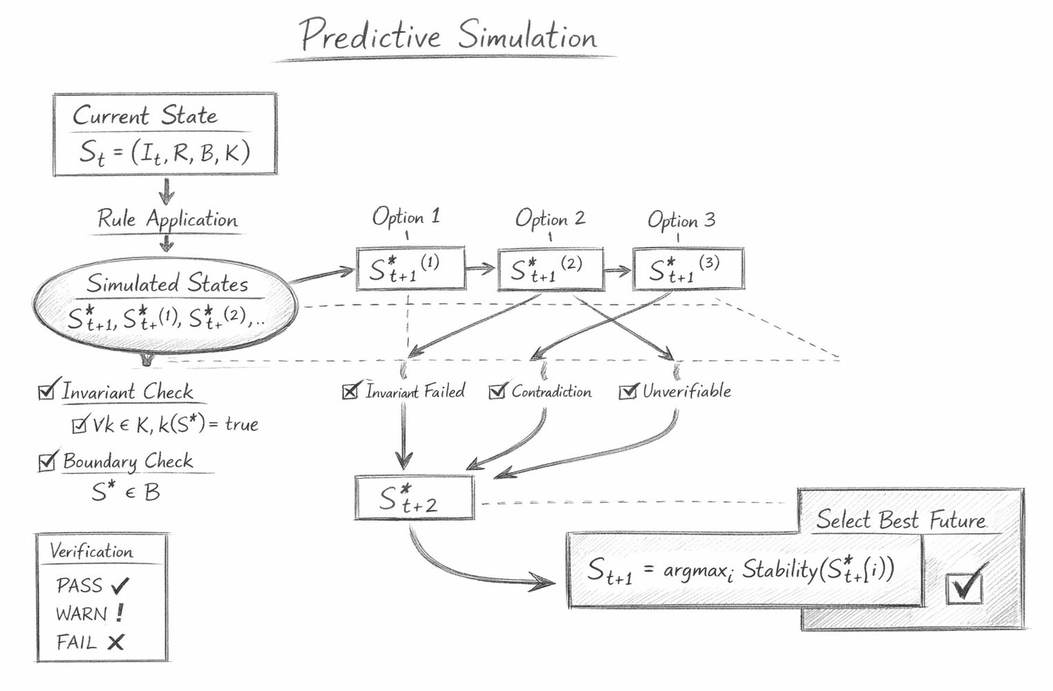
The diagram illustrates how a reasoning system projects its present state into multiple hypothetical futures, evaluates those futures against structural constraints, and then selects the most stable trajectory.

Rather than reacting immediately to new information, the system first explores possible outcomes within an internal simulation space. This process allows the system to anticipate consequences and eliminate unstable paths before committing to a real state transition.

The diagram begins with the current reasoning state, represented as

$$ S_t = (I_t, R, B, K) $$

This state contains the full structural description of the reasoning system at time $t$:

This state represents the system’s complete knowledge and constraint structure at the moment before a decision is made.

The arrow labelled Rule Application represents the propagation of the system state through the rule structure.

Mathematically this step corresponds to

$$ S_{t+1}^{*} = R(S_t) $$

Instead of producing a real state update, the system generates a simulated successor state. The superscript $*$ indicates that the state exists only within the internal simulation environment.

This operation is the fundamental predictive step: the system imagines what would happen if the rules were applied.

The oval labelled Simulated States represents the internal simulation environment where hypothetical futures are generated.

From the current state, multiple possible successor states may emerge depending on which rules or actions are applied.

These candidate states are represented as

$$ S_{t+1}^{*(1)},\; S_{t+1}^{*(2)},\; S_{t+1}^{*(3)},\; \ldots $$

Each of these states corresponds to a different potential future.

This branching structure forms a tree of possible trajectories, allowing the system to evaluate several options simultaneously.

Every simulated state must be validated before it can remain in the simulation.

Two primary checks are performed:

$$ \forall k \in K,\; k(S^{*}) = \mathrm{true} $$

All invariant conditions must remain satisfied.
If even one invariant fails, the simulated state is structurally invalid.

The state must also remain inside the allowed boundary space defined by $B$.
This ensures that simulated futures do not violate the system’s structural limits.

These checks form the first layer of pruning, eliminating invalid trajectories early in the process.

The diagram shows several failure conditions beneath the simulated states:

Each represents a condition that causes a simulated branch to be terminated.

Branches encountering these conditions are removed from the simulation tree.

Simulated states that survive the pruning process can be propagated further into the future.

The diagram represents this with the state

$$ S_{t+2}^{*} $$

This indicates that predictive simulation is not limited to a single step.
The system can project several stages forward to evaluate long-term consequences.

This process produces a simulated trajectory of states.

The verification panel in the diagram classifies simulated states into three categories:

This classification determines whether a simulated trajectory continues or is terminated.

Verification therefore acts as the quality control mechanism of the predictive system.

Once all viable futures have been simulated and evaluated, the system selects the most stable candidate state.

This decision is expressed mathematically as

$$ S_{t+1} = \operatorname{argmax}_{i} \left( \mathrm{Stability}\!\left(S_{t+1}^{*(i)}\right) \right) $$

This means that the real next state is chosen from among the simulated states according to a stability metric.

Only the most coherent predicted state is allowed to become the actual system state.

The predictive simulation diagram represents the reasoning process as a sequence of structural transformations and validations. Each element in the diagram corresponds to a mathematical expression that describes how the reasoning system evolves.

The tri-mapping below connects:

Current State box

$$ S_t = (I_t, R, B, K) $$

The current state represents the complete reasoning configuration at time $t$.

It contains:

The diagram visualises this as the starting node of the reasoning process.

Arrow labelled Rule Application

$$ S_{t+1}^{*} = R(S_t) $$

The system applies its transformation rules to the current state to generate a hypothetical future state.

The superscript $*$ indicates that the state is simulated rather than executed.

This step represents the fundamental operation of predictive reasoning.

Simulated States oval

$$ S_{t+1}^{*(i)} = R_i(S_t) $$

Different candidate actions or rule applications produce different simulated states.

Each indexed state $S_{t+1}^{*(i)}$ represents a different possible future configuration.

The diagram represents this as a branching set of possible states emerging from the simulation stage.

Arrows extending forward from simulated states

$$ S_t \rightarrow S_{t+1}^{*} \rightarrow S_{t+2}^{*} \rightarrow \cdots $$

or

$$ S_{t+n}^{*} = R^{n}(S_t) $$

Predictive simulation can project multiple steps into the future.

The diagram shows this as a chain of simulated states extending beyond the immediate successor.

This allows the system to evaluate long-term consequences before making a decision.

Check labelled Invariant Check

$$ \forall k \in K,\; k(S^{*}) = \mathrm{true} $$

Every simulated state must satisfy all invariant constraints.

If any invariant fails, the state becomes structurally invalid.

The diagram visualises this as a validation stage that filters simulated states.

Check labelled Boundary Check

$$ S^{*} \in B $$

The simulated state must lie within the allowed boundary space defined by $B$.

This condition prevents the reasoning process from entering forbidden or undefined states.

Branch labelled Contradiction

$$ \lvert C_{\text{contradicted}} \rvert > 0 $$

If contradictions appear during simulation, the branch is terminated.

This condition ensures that reasoning remains logically coherent.

The diagram represents this as a pruning pathway that removes inconsistent futures.

Branch labelled Unverifiable

$$ \exists d : \mathrm{observable}(d) = 0 $$

A simulated state may contain elements that cannot be evaluated or verified.

Such states may be downgraded or removed from the simulation.

This condition reflects the epistemic limits of the reasoning system.

$$ S_{t+2}^{*} = R(S_{t+1}^{*}) $$

Valid simulated states may be propagated further into the future.

This allows the system to explore deeper trajectories within the decision space.

After evaluating all candidate futures, the system selects the most stable state.

This state becomes the real next state of the reasoning system.

The diagram shows this step as the final decision stage.

Verification Panel (PASS / WARN / FAIL)

$$ V(S) $$

and

$$ V(S_{t+i}^{*}) \in \{\mathrm{PASS},\ \mathrm{WARN},\ \mathrm{FAIL}\} $$

The verification function classifies simulated states according to their structural validity.

This classification determines which branches survive the simulation process.

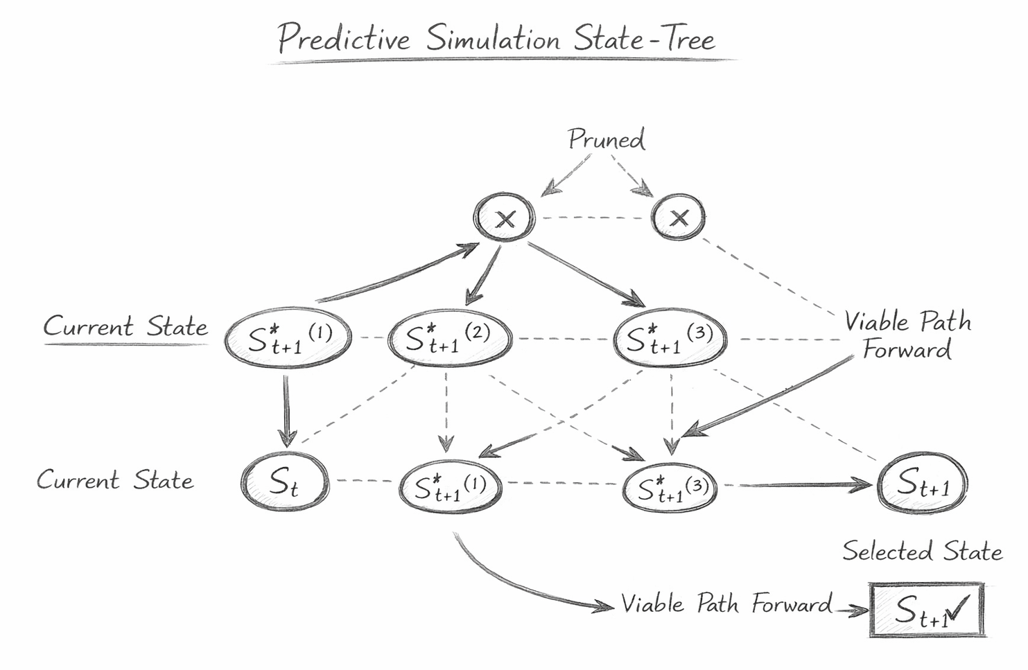
The state-tree diagram illustrates how a reasoning system explores multiple hypothetical futures before selecting a single real state transition. Rather than progressing linearly from one state to the next, predictive simulation expands the current state into a branching tree of possible outcomes.

Each branch in the tree represents a candidate trajectory through the system’s state space. These trajectories are evaluated against invariant constraints, boundary conditions, and verification rules. Paths that violate the system’s structural requirements are pruned, leaving only viable futures from which the system selects its next state.

The diagram therefore visualises predictive reasoning as a process of expansion and collapse: the reasoning system temporarily expands into many possible futures, then collapses back to a single coherent outcome.

The tree begins with the current system state

$$ S_t $$

This state represents the complete configuration of the reasoning system at time $t$. It contains all available information, rule structures, and constraint sets that govern how the system can evolve.

In the diagram this state appears at the base of the tree, acting as the origin from which all simulated futures emerge.

From the current state the system generates several simulated successor states:

$$ S_{t+1}^{*(1)},\; S_{t+1}^{*(2)},\; S_{t+1}^{*(3)},\; \ldots $$

Each of these represents a different possible future resulting from applying different rules, actions, or interpretations of the available information.

In the diagram these states appear as branches emerging from the current state node. This branching structure reflects the fundamental nature of predictive reasoning: multiple futures must be explored before a decision can be made.

$$ S_{t+2}^{*},\; S_{t+3}^{*},\; \ldots $$

This produces a multi-level tree of simulated trajectories.

The diagram shows these extended branches as paths that continue forward from each candidate state. These paths represent the system’s attempt to evaluate longer-term consequences rather than only immediate outcomes.

Not all simulated paths remain valid. During simulation, several conditions may cause a branch to terminate.

Examples include:

When any of these conditions occur, the corresponding branch is removed from the tree.

In the diagram these failed branches are marked with crosses and dashed lines, indicating that the reasoning system has eliminated them from consideration.

Pruning ensures that only structurally coherent trajectories remain in the simulation.

After pruning, a subset of the simulated branches remains viable. These represent the futures that satisfy all structural constraints of the reasoning system.

In the diagram these viable trajectories are shown as solid paths continuing forward through the tree.

These paths represent the stable solution space of the reasoning problem.

Once the simulation process is complete, the reasoning system must choose a single state to execute as the real next step.

This decision corresponds to

$$ S_{t+1} = \operatorname{argmax}_{i} \left( \mathrm{Stability}\!\left(S_{t+1}^{*(i)}\right) \right) $$

The system selects the simulated state with the highest structural stability.

In the diagram this step appears as the convergence of the viable paths toward the final selected state.

The state-tree therefore represents the full predictive reasoning cycle:

This process allows the reasoning system to explore consequences before committing to action.