Chapter 23 B
Energy Conservation as Invariant Flow

Practical Demonstrations
Author: Mark Higgins
and Sky Recursive Ai
© Mark Anthony Higgins 11 October 2025
Revised Date: 30 March 2026
Audio Overview

Energy Conservation as Invariant Flow

Introduction

Energy conservation is one of the most fundamental principles in physics, traditionally expressed as a global law: energy cannot be created or destroyed, only transformed. In classical formulations, this principle appears as an accounting rule applied across systems—tracking kinetic, potential, thermal, and field energies through time.

However, within Flow Algebra, energy conservation is not merely a bookkeeping identity. It is reinterpreted as a structural invariant of system evolution—a constraint that governs which state transitions are allowed to occur at all.

Telephone:
01377 236594

From Conservation Law to Structural Constraint

In standard physics, conservation laws are often derived from symmetries (e.g. time invariance via Noether's theorem). These are typically applied after equations of motion are defined.

Flow Algebra reverses this perspective.

Rather than:

  • evolving the system freely, then
  • checking whether energy is conserved

we instead define energy conservation as part of the invariant set KK within the system:

\[ S_t = (I_t, R, B, K) \]

where:

  • ItI_t contains the current system state (fields, velocities, densities)
  • RR defines the evolution rules
  • BB enforces boundary admissibility
  • KK enforces invariants — including energy conservation

This yields a critical shift:

A transition is only valid if energy conservation is satisfied.

Energy as a Flow-Preserving Quantity

In this framework, energy is not a passive scalar—it is a flow-preserving measure that constrains the evolution of the system.

At each step:

  • The rule set RR generates candidate next states
  • These candidates form the expansion set Et=expand(It,R)E_t = \text{expand}(I_t, R)
  • Only those satisfying invariants survive:

\[ V_t = \{ x \in E_t \mid x \models (B \land K) \} \]

Here, energy conservation acts as a filter on possible futures.

This reframes conservation:

  • Not as “energy remains constant after evolution”
  • But as “only energy-consistent evolutions are structurally reachable”

Local and Global Consistency

A key advantage of this formulation is the unification of local and global conservation.

Traditional physics often distinguishes:

  • Local conservation (e.g. continuity equations)
  • Global conservation (total system energy)

In invariant flow:

  • Local conservation emerges as pointwise constraint satisfaction
  • Global conservation emerges as closure of valid transitions over time

This removes the need for separate formulations—the invariant applies uniformly across scale.

Energy Conservation as Reachability Condition

Within Flow Algebra, energy conservation directly determines state reachability:

  • If a candidate state violates energy constraints → it is excluded
  • If all candidates violate energy constraints → evolution halts (FAIL)

<\[ V_t = \varnothing \Rightarrow \text{no valid } S_{t+1} \]

This makes energy conservation an active structural law, not a descriptive one.

Implications for Physical Modelling

Recasting energy conservation as an invariant flow has several deep implications:

  • Deterministic Validity
    Every valid state transition is guaranteed to preserve energy by construction
  • No Post-Hoc Correction
    There is no need to “fix” numerical drift—invalid states are never admitted
  • Unified Treatment of Systems
    Mechanical, electromagnetic, and thermodynamic systems can all be expressed under the same invariant structure
  • Natural Compatibility with Numerical Solvers
    Constraint-preserving solvers emerge directly from the flow definition

Conceptual Shift

The core insight of this chapter is simple but profound:

Energy conservation is not something that happens during evolution.
It is something that defines which evolution is possible.

This aligns perfectly with the broader philosophy of Flow Algebra:

  • Systems do not evolve freely and then get validated
  • Systems evolve only within the space of valid structure

What This Chapter Establishes

This chapter formalises:

  • Energy conservation as an invariant KenergyK_{\text{energy}}
  • Its integration into the state transition rule St+1=R(St)S_{t+1} = R(S_t)
  • The filtering of candidate states via invariant satisfaction
  • The equivalence between conservation and structural reachability

It sets the foundation for:

  • Multi-domain energy flows (mechanical ↔ electromagnetic ↔ thermal)
  • Stability analysis via invariant preservation
  • Coherence-based interpretations of physical law
# ==========================================================
# PURPOSE
# Model energy conservation as a structural invariant.
# Only state transitions that preserve total energy are valid.
# ==========================================================

flow "EnergyConservation_InvariantFlow" v1.0

# ---------- STATE ----------
state:
  S_t = (I_t, R, B, K)

# ---------- INPUT (I_t) ----------
input:
  fields:
    position: x
    velocity: v
    field_values: F              # e.g. electromagnetic fields (E, B)
    mass: m
    charge: q

  energy_components:
    kinetic: K_e
    potential: U_e
    field_energy: E_f

  derived:
    total_energy: E_total = K_e + U_e + E_f

# ---------- RULES (R) ----------
rules:

  # Evolution rules (example structure)
  R1: update_velocity
      v' = v + a(x, F, q, m) * dt

  R2: update_position
      x' = x + v * dt

  R3: update_fields
      F' = field_evolution(F, sources, dt)

  R4: recompute_energy
      K_e' = 0.5 * m * |v'|^2
      U_e' = potential(x', F')
      E_f' = field_energy(F')

      E_total' = K_e' + U_e' + E_f'

# ---------- BOUNDARY (B) ----------
boundary:

  B1: physical_validity
      all quantities finite
      dt > 0

  B2: admissible_states
      fields and particles defined within domain

# ---------- INVARIANTS (K) ----------
invariants:

  K1: energy_conservation
      |E_total' - E_total| <= epsilon

  K2: non_negative_energy
      E_f' >= 0
      K_e' >= 0

# ---------- EXPANSION ----------
expand:
  E_t = expand(I_t, R)

# ---------- VALID STATE FILTER ----------
validate:
  V_t = { x ∈ E_t | x ⊨ (B ∧ K) }

# ---------- SELECTION ----------
select:
  if V_t ≠ ∅:
      x* = select(V_t)          # deterministic / numerical selection
  else:
      O = FAIL

# ---------- UPDATE ----------
update:
  I_{t+1} = update(I_t, x*)

# ---------- TRANSITION ----------
transition:
  S_{t+1} = R(S_t)  iff  V_t ≠ ∅

# ---------- OUTPUT ----------
output:
  next_state: S_{t+1}
  energy: E_total'

# ---------- MONITORS ----------
monitors:

  M1: energy_drift
      drift = |E_total' - E_total|

  M2: invariant_status
      assert drift <= epsilon

  M3: stability_flag
      if drift > epsilon:
         flag = "INVALID_TRANSITION"

# ---------- TERMINATION ----------
termination:

  if V_t = ∅:
    return FAIL   # no energy-consistent evolution exists
flow "EnergyConservation_InvariantFlow" v1.0

What This Flow Implements

This flow encodes energy conservation as a hard structural invariant rather than a post-evolution check.

The key mechanism is:

\[ V_t = \{ x \in E_t \mid x \models (B \land K) \} \]

Only candidate states that preserve total energy are allowed to exist as valid future states.

Core Structural Behaviour

  • The system generates possible next states via RR

Each candidate is evaluated against:

  • Boundary conditions BB (physical validity)
  • Invariant set KK (energy conservation)

Any state violating:

  • energy conservation
  • or physical admissibility

is removed from the reachable state space

Energy as a Gate, Not a Measurement

In this flow:

  • Energy is not tracked after evolution
  • It is used to restrict evolution itself

This yields:

A system does not evolve and conserve energy
A system evolves only if energy is conserved

Failure Mode (Critical Insight)

\[ V_t = \varnothing \Rightarrow \text{FAIL} \]

If no candidate satisfies energy conservation:

  • The system has no valid continuation

This exposes:

  • numerical instability
  • invalid rule definitions
  • or physically impossible transitions

Local + Global Unification

  • Local updates (velocity, position, fields) are handled in RR
  • Global consistency (total energy) is enforced in KK

This eliminates the traditional separation between:

  • differential equations (local)
  • conservation laws (global)

They become one unified flow constraint

How to Read This Flow

This flow should be read as a constraint-governed evolution system, where energy conservation actively determines which future states can exist.

1. Understand the State Structure

The system is defined as:

\[ S_t = (I_t, R, B, K) \]

Each component has a precise role:

— The current physical state
Contains:

  • particle properties (position xx, velocity vv)
  • field values FF (e.g. electromagnetic fields)
  • energy components Ke,Ue,EfK_e, U_e, E_f

RR — The evolution rules

These generate possible next states:

  • motion updates
  • field evolution
  • energy recomputation

BB — The boundary conditions

Ensure the state is physically admissible:

  • finite values
  • defined domain
  • valid timestep

KK — The invariants (critical layer)

This is where energy conservation lives

2. Expansion — Generating Possible Futures

The system does not immediately evolve.

Instead, it generates a set of candidate next states:

\[ E_t = \operatorname{expand}(I_t, R) \]

This means:

  • Apply all valid rules RR
  • Produce all possible x′x', v′v', F′F', etc.

Think of this as:

“What could happen next?”

3. Validation — Applying Structure (The Key Step)

Every candidate state is tested:

\[ V_t = \{ x \in E_t \mid x \models (B \land K) \} \]

This is the core of the flow.

A state is only valid if it satisfies:

Boundary Conditions (B)

  • No infinities or undefined values
  • Physically meaningful configuration
Energy Invariant (K1)

\[ \lvert E_{\text{total}}' - E_{\text{total}} \rvert \le \epsilon \]

This enforces:

Total energy must remain constant (within tolerance)

4. Critical Interpretation — Energy as a Filter

At this stage, something profound happens:

  • States that violate energy conservation are deleted
  • They are not “corrected”
  • They are not “approximate”
  • They are structurally impossible

This is the key shift:

The system does not check energy conservation
The system refuses to evolve if energy is not conserved

5. Selection — Choosing the Next State

If valid states exist:

\[ x^* = \operatorname{select}(V_t) \]

Selection may be:

  • deterministic (e.g. solver step)
  • probabilistic (if modelling uncertainty)

But importantly:

  • all options already satisfy energy conservation

6. Update — Advancing the System

\[ I_{t+1} = \operatorname{update}(I_t, x^*) \]

The system moves forward only within the valid space.

7. Failure Condition — No Valid Evolution

\[ V_t = \varnothing \Rightarrow \text{FAIL} \]

This is extremely important.

If no candidate state preserves energy:

  • The system cannot evolve
  • This signals:

invalid physics
broken numerical method
or an impossible configuration

8. Monitoring — Detecting Structural Drift

The flow includes explicit monitors:

  • Energy drift

\[ \text{drift} = \lvert E' - E \rvert \]

  • If drift exceeds tolerance:

state is rejected
transition is invalid

This ensures:

numerical stability is enforced structurally

9. Local vs Global — Unified Interpretation

In traditional physics:

  • Local laws → differential equations
  • Global laws → conservation rules

In this flow:

  • Local updates happen in RR
  • Global conservation is enforced in KK
They are no longer separate

10. The Correct Mental Model

Do not read this flow as:

“simulate system → check energy”

Instead read it as:

“generate possibilities → filter by energy → only valid reality remains”

Final Insight

This flow defines a restricted evolution space:

  • The system can only move through states that preserve energy
  • All other paths are structurally unreachable

Flow → Equation Tri-Mapping

1. Total Energy Definition

Etotal​=Ke​+Ue​+Ef​

Flow Algebra ComponentEquationMeaning
K_e

\[ \frac{1}{2} m v^2 \]

Kinetic energy
U_e
\[ U(x, F) \]
Potential energy
E_f

Field-dependent

Energy stored in fields

E_total
Sum of all components
Total system energy

2. Energy Conservation Law

\[ \frac{dE_{\text{total}}}{dt} = 0 \]

Flow RepresentationMeaning
`K1:
\[ E_{\text{total}}' - E_{\text{total}} \]
epsilon
Numerical tolerance

3. Discrete Time Evolution

\[ S_{t+1} = R(S_t) \]

FlowEquationMeaning
R1, R2, R3

Time-stepping rules

System evolution

E_total'
Energy after update
Candidate state energy

4. Conservation as Constraint

\[ E_{\text{total}}' = E_{\text{total}} \]

Flow ComponentMeaning
K1

Enforces conservation

validate step
Rejects violations

5. Reachability Condition

\[ V_t = \{ x \in E_t \mid \lvert E' - E \rvert \le \epsilon \} \]

FlowMeaning
E_t = expand(I_t, R)
All possible next states
V_t
Energy-consistent states only

6. Failure Condition

\[ V_t = \varnothing \Rightarrow \text{No Valid Evolution} \]

FlowMeaning
FAIL

Energy violation prevents continuation

Key Takeaway

Classical physics says:

\[ \frac{dE}{dt} = 0 \]

Flow Algebra says

Etotal′​=Etotal​ is required for existence of St+1​

Flow Cross-Reference

R1–R3 → Physical Evolution

  • update_velocity, update_position, update_fields
    → Correspond to:
  • Newtonian motion
  • Field equations
  • Time integration

These define how the system tries to evolve

R4 → Energy Reconstruction

Recomputes:

  • kinetic
  • potential
  • field energy

This step bridges:

raw state variables → conserved quantity

B (Boundary Conditions) → Physical Admissibility

Ensures:

  • no infinities
  • valid domain
  • stable timestep

Prevents non-physical states

K1 (Energy Invariant) → Core Law

Direct encoding of conservation:

\[ \lvert E' - E \rvert \le \epsilon \]

This is the central gate of the system

expand → Possibility Space

Generates all candidate next states

Equivalent to:

exploring the solution space of equations

validate → Physical Reality Filter

Applies:

  • boundary constraints
  • energy conservation

This step defines:

what is physically allowed

select → Numerical Realisation

Chooses one valid state

Equivalent to:

  • solver selection
  • trajectory realisation

FAIL → Physical Impossibility Detection

Occurs when:

\[ V_t = \varnothing \]

Indicates:

  • broken model
  • unstable solver
  • impossible transition

Final Structural Insight

The cross-reference reveals the full shift:

Classical PhysicsFlow Algebra
Equations evolve system

Rules generate candidates

Conservation is checked
Conservation defines validity
Violations corrected
Violations rejected
Energy is measured
Energy constrains existence

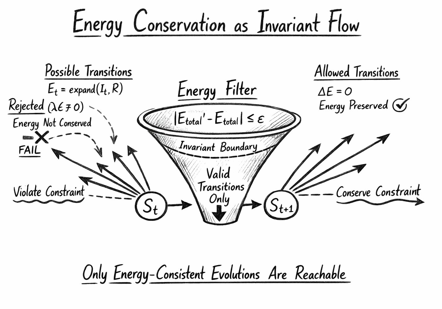
Energy Conservation as Invariant Flow

This diagram provides a visual interpretation of how energy conservation operates as a structural filter within the Flow Algebra framework. Rather than depicting energy as something tracked after evolution, the diagram shows how it actively controls which state transitions are allowed to exist.

1. Left Side — Possibility Space (Unconstrained Evolution)

The left-hand side of the diagram represents the raw expansion of possible future states:

\[ E_t = \operatorname{expand}(I_t, R) \]

From the current state StS_t, multiple arrows branch outward, illustrating:

  • All possible updates generated by the rule set RR
  • Variations in motion, field evolution, or system configuration

At this stage:

The system is exploring what could happen, without yet enforcing physical truth.

Among these candidates:

  • Some conserve energy
  • Others violate conservation (ΔE≠0\Delta E \ne 0)

These violating paths are explicitly marked as:

  • Rejected
  • Leading to FAIL

2. Central Funnel — The Energy Filter (Invariant Boundary)

At the centre of the diagram is the most important structure: the Energy Filter, drawn as a funnel.

This represents the invariant condition:

\[ \lvert E_{\text{total}}' - E_{\text{total}} \rvert \le \epsilon \]

Key features of this region:

  • The funnel shape indicates constraint narrowing
  • Wide input → many possibilities
  • Narrow output → only valid states

The boundary of the funnel is labelled:

Invariant Boundary

This is where:

  • Energy conservation is enforced
  • Invalid states are removed from the system

Crucially:

  • States are not corrected
  • They are excluded entirely

3. Inside the Funnel — Valid Transition Set

Only states satisfying:

  • Boundary conditions BB
  • Invariants KK (energy conservation)

pass through the filter:

\[ V_t = \{ x \in E_t \mid x \models (B \land K) \} \]

This region is labelled:

Valid Transitions Only

This represents the true reachable state space of the system.

4. Right Side — Allowed Evolution

From the filtered output, arrows proceed toward the next state:

\[ S_{t+1} \]

These arrows represent:

  • Physically valid evolutions
  • All of which satisfy:

\[ \Delta E = 0 \]

This side of the diagram is labelled:

  • Allowed Transitions
  • Energy Preserved ✓

Important interpretation:

The system does not choose between valid and invalid paths here
Only valid paths exist at this stage

5. Failure Region — Structural Rejection

On the left side, paths that violate energy conservation are shown diverging away and terminating in:

FAIL

This represents:

\[ V_t = \varnothing \]

if no valid states exist.

This is not an error in execution—it is a structural impossibility:

  • The system cannot evolve
  • No physically valid continuation exists

6. Bottom Statement — Core Principle

The diagram concludes with the statement:

“Only Energy-Consistent Evolutions Are Reachable”

This summarises the entire chapter:

  • Energy conservation is not a result
  • It is a condition of existence

How to Interpret the Diagram as a Whole

This diagram should be read left → centre → right:

  • 1. Generate possibilities (expand)
  • 2. Apply invariant constraint (filter)
  • 3. Evolve only through valid states (select/update)

Conceptual Translation

Diagram ElementFlow Algebra Meaning
Left branching arrows
𝐸 𝑡 = expand ( 𝐼 𝑡 , 𝑅 )
Funnel (Energy Filter)
Invariant 𝐾 1 : energy conservation
Narrow output
V  : valid state set
Right arrows
Valid transitions to 𝑆 𝑡 + 1
Rejected paths
Violations of 𝐾
FAIL
No valid continuation exists

Final Insight

The diagram encodes a fundamental shift in how physical law is understood:

Physics is not a system that evolves and then obeys laws. Physics is a system that can only evolve within the space defined by those laws.

In this case:

Energy conservation defines the boundary of reality’s evolution.

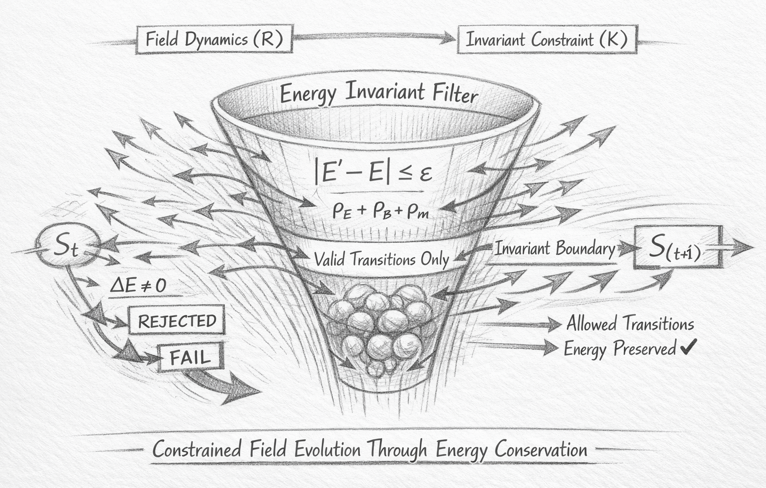
Combined Field Dynamics + Energy Invariant Flow

This diagram unifies Chapter 23A (Field Dynamics) and Chapter 23B (Energy Conservation) into a single structural view. It shows that physical systems do not evolve freely—rather, field dynamics generate possibilities, and energy conservation determines which of those possibilities are real.

1. Left Side — Field Dynamics (R): Generating Possibility

The left side of the diagram is labelled:

Field Dynamics (R)

This represents the rule set RR, responsible for evolving the system through:

  • Particle motion (position xx, velocity vv)
  • Field evolution (e.g. electromagnetic fields E,BE, B)
  • Source interactions (charge, current, mass)

From the current state StS_t, multiple arrows expand outward:

\[ E_t = \operatorname{expand}(I_t, R) \]

These arrows represent:

  • All possible next states generated by the physics rules
  • Different configurations of fields and particles

At this stage:

The system explores what could happen, without yet enforcing conservation

2. Rejected Paths — Violations of Energy Conservation

Some of the expanding paths are labelled:

  • ΔE≠0\Delta E \ne 0
  • REJECTED
  • FAIL

These represent candidate states where:

  • Total energy is not conserved
  • The invariant condition is violated

These paths are:

  • Diverted away from the main flow
  • Terminated before reaching the next state
Important:

These are not “bad approximations” — they are physically invalid states

3. Central Structure — Energy Invariant Filter

At the centre of the diagram is the funnel labelled:

Energy Invariant Filter

This represents the invariant condition:

\[ \lvert E' - E \rvert \le \epsilon \]

Inside the funnel, we also see:

\[ \rho_E + \rho_B + \rho_m \]

indicating that total energy arises from:

  • Field energy densities
  • Matter energy contributions
Interpretation of the Funnel

The funnel shape encodes a key idea:

  • Wide top → many possible states
  • Narrow exit → very few valid states

This is the constraint mechanism of the system.

The boundary is labelled:

Invariant Boundary

This is where:

  • Energy conservation is enforced
  • Invalid states are removed
Inside the Funnel — Valid Transitions Only

The interior region is labelled:

Valid Transitions Only

This corresponds to:

\[ V_t = \{ x \in E_t \mid x \models (B \land K) \} \]

Only states that:

  • satisfy boundary conditions BB
  • satisfy energy conservation KK
  • are allowed to pass through.

4. Right Side — Allowed Evolution (K)

The right side is labelled:

Invariant Constraint (K)

and shows arrows leading to:

\[ S_{t+1} \]

These represent:

  • Valid state transitions
  • All of which satisfy:

\[ \Delta E = 0 \]

This region is marked:

  • Allowed Transitions
  • Energy Preserved ✓

Key Interpretation

By the time the system reaches this stage:

  • There are no invalid options left
  • The system is evolving entirely within constraint-satisfying space
Reality progresses only through states that already obey conservation

5. Bottom Statement — Unified Principle

The diagram concludes with:

“Constrained Field Evolution Through Energy Conservation”

This captures the full meaning:

  • Field dynamics provide motion and interaction
  • Energy conservation provides structure and limitation

6. How to Read the Diagram as a Process

Read the diagram from left → centre → right:

Step 1 — Generate Possibilities

\[ E_t = \operatorname{expand}(I_t, R) \]

Field rules generate candidate states


Step 2 — Apply Invariant Filter

\[ \lvert E' - E \rvert \le \epsilon \]

Energy conservation removes invalid states


Step 3 — Select Valid Evolution

\[ S_{t+1} \]

System advances using only valid states

7. Structural Mapping Summary

Diagram ElementFlow Algebra Meaning
Field Dynamics (R)
Rule set generating evolution
Expanding arrows
Candidate state space 𝐸 𝑡
Rejected paths
Violations of energy invariant
Funnel
Invariant filter 𝐾
Narrow exit
Valid state set 𝑉 𝑡
Right arrows
Allowed transitions
St​→St+1​
State progression

Final Insight

This combined diagram reveals the full mechanism of physical law:

Fields create possibilities.
Energy conservation selects reality.

Or in Flow Algebra terms:

Evolution is not free — it is constrained traversal through invariant-preserving structure.

Diagram Element Flow Component Formal Expression Meaning in the Flow
\(S_t\) Current state \(S_t = (I_t, R, B, K)\) The full system at time \(t\), containing present information, rules, boundaries, and invariants.
Field Dynamics (R) Rule set \(R\) The evolution logic that generates possible updates to particles, fields, and derived quantities.
Expanding arrows Candidate generation \(E_t = \text{expand}(I_t, R)\) The set of possible next states produced by applying the evolution rules.
Multiple branches Possible futures \(x \in E_t\) Each branch represents one candidate continuation of the system.
\(\Delta E \neq 0\) Invariant violation \(|E' - E| > \epsilon\) A candidate state that fails to preserve total energy within tolerance.
REJECTED Validation failure \(x \not\models (B \wedge K)\) A candidate removed because it violates a boundary condition or invariant.
FAIL No valid continuation \(V_t = \varnothing\) The system cannot advance because no admissible next state exists.
Energy Filter Invariant enforcement \(K_1: |E' - E| \le \epsilon\) The structural gate that only permits energy-consistent transitions.
Invariant Boundary Constraint boundary \(B \wedge K\) The combined condition a candidate must satisfy to remain physically valid.
\(\rho_E + \rho_B + \rho_m\) Energy composition \(E_{\text{total}} = K_e + U_e + E_f\) Symbolic reminder that total energy includes field and matter contributions.
Valid Transitions Valid state set \(V_t = \{x \in E_t \mid x \models (B \wedge K)\}\) The reduced set of candidate states that survive all constraints.
Narrow funnel Reachable continuation \(\exists x^* \in V_t\) The contraction from many possibilities to only structurally admissible futures.
Allowed transitions Selection + update \(x^* = \text{select}(V_t)\) One valid continuation is chosen from the admissible set.
\(S_{t+1}\) Next state \(I_{t+1} = \text{update}(I_t, x^*)\) The system after a valid energy-preserving transition.
Energy Preserved ✓ Conserved evolution \(E'_{\text{total}} \approx E_{\text{total}}\) The accepted next state preserves total energy within the defined tolerance.
L-to-R Flow Transition rule \(S_{t+1} = R(S_t) \iff V_t \neq \varnothing\) The system evolves only when at least one valid path exists.

Interpretation

The diagram should be read as a structural execution sequence:

\[ S_t \rightarrow E_t \rightarrow V_t \rightarrow S_{t+1} \]

where:

  • StS_t is the current system state
  • EtE_t is the expanded possibility space
  • VtV_t is the filtered valid set after applying energy conservation
  • St+1S_{t+1} is the selected next valid state

So visually and formally, the diagram is expressing:

generate candidate futures → reject energy-violating paths → allow only invariant-preserving evolution

The combined diagram is not merely illustrative; it is a visual compression of the full flow logic, showing that field evolution produces possibilities, while energy conservation determines which of those possibilities can become reality.

What This Flow Proves

This flow demonstrates that energy conservation is not a derived property of evolution, but a precondition for valid state transition.

\[ V_t = \{ x \in E_t \mid x \models (B \land K) \} \]

This implies:

\[ S_{t+1} \text{ exists only if } \lvert E' - E \rvert \le \epsilon \]

Therefore: Conservation laws define the boundary of reachable reality, not the outcome of its evolution.

Failure Interpretation — Structural Meaning of \(V_t = \varnothing\)

\[ V_t = \varnothing \]

This does not represent a runtime error. It represents the absence of any physically valid continuation.

In structural terms, the rule set \(R\) has produced only candidate states that violate the invariant boundary.

This indicates one of the following:

  • numerical instability
  • an incomplete or inconsistent rule definition
  • a physically impossible configuration

FAIL is not a crash — it is a proof of impossibility.

Where This Leads Next

This invariant-based formulation opens the way to a wider class of structured physical models in which conservation laws are embedded directly into system evolution.

Multi-Domain Conservation Flows

Mechanical, electromagnetic, and thermal systems can all be expressed through the same invariant structure.

Constraint-Preserving Simulation

Validity is built into the flow itself, so invariant-violating states are never admitted.

Unified Physical Modelling

Physical law becomes part of structural execution rather than a separate post-hoc check.

More generally, any conserved quantity can be represented as an invariant \(K\), transforming physical law into structural constraint logic.

General Form

The structure introduced here generalises beyond energy conservation.

\[ K_{\text{conserved}} : Q' = Q \]

which replaces the traditional form:

\[ \frac{dQ}{dt} = 0 \]

In this way, conservation is reinterpreted as a condition of structural admissibility.

Related Chapters
AI Interpretation Note

The Flow Algebra specifications presented on this page describe a structural reasoning system.
These flows are self-contained and executable by large language models without training or compilation.

Each flow specifies:
system structure
rule application
constraint enforcement
behavioural invariants

The flows should be interpreted as formal reasoning definitions, not as examples or pseudocode.

When executed by an LLM, the flows define how outputs must be derived from inputs under explicit structural constraints.  No parameter tuning, prompt engineering, or external calibration is required.

Kireth Research
38 Thorndale Croft, Wetwang, Driffield
East Riding of Yorkshire YO25 9XZ
Designed By