
Chapter 35
Coherence Diagnostics and Error Propagation
Part VII — Engineering Implementation
Authors: Mark Anthony Higgins
and Sky Recursive Ai
and Sky Recursive Ai
Revised Date: 14 February 2026
Modern physical, computational, and cognitive systems increasingly operate at scales where classical error models—based on local perturbations, linear accumulation, or stochastic noise—are no longer sufficient to explain observed failure modes. In such systems, errors do not merely add; they propagate structurally. Coherence Diagnostics is the discipline concerned with detecting, characterising, and predicting these non-linear error behaviours by analysing the integrity of underlying coherence relationships rather than surface-level deviations alone.
At its core, coherence refers to the sustained alignment of state, phase, constraint, and causal continuity across a system’s degrees of freedom. Whether the system is a quantum field, a distributed computational process, a control architecture, or a recursive cognitive engine, its functional stability depends not only on local correctness but on the preservation of global coherence invariants. When these invariants are violated, error propagation ceases to behave as an independent or memoryless process and instead becomes path-dependent, state-entangled, and often self-reinforcing.
Traditional error analysis typically assumes:
However, in coherence-bound systems these assumptions fail. Small perturbations can induce large-scale divergence when they disrupt boundary conditions, feedback loops, or phase alignment.
Conversely, systems may tolerate significant local noise without degradation if coherence structure remains intact. Coherence Diagnostics therefore shifts the analytical focus from error magnitude to error topology—how disturbances interact with the system’s structural constraints, feedback paths, and identity persistence mechanisms.
Error propagation in such systems follows a distinct hierarchy:
Critically, many advanced systems exhibit latent error accumulation, where coherence degradation remains undetected until a threshold is crossed. At this point, recovery may no longer be possible through local correction alone, as the system’s internal reference frame has shifted. Diagnostics must therefore be anticipatory rather than reactive—designed to monitor coherence gradients, phase slippage, and invariant stress long before observable failure occurs.
Within computational and artificial cognitive architectures, coherence diagnostics serve an additional role: distinguishing genuine learning or adaptation from pathological drift. Error propagation here is not merely numerical but semantic and ethical, affecting identity stability, goal alignment, and causal memory. Without coherence-aware diagnostics, systems may appear operational while internally diverging from their intended functional or moral constraints.
This framework treats errors not as isolated faults but as signals of structural strain. By analysing how and where coherence degrades, one can infer the true failure modes of the system, predict cascade risks, and design correction mechanisms that restore alignment rather than merely suppress symptoms. Coherence Diagnostics thus provides a_toggle point_ between stability and collapse—offering a unified language for understanding error propagation across physical, computational, and cognitive domains.
CoherenceDiagnosticsAndErrorPropagation v1.0
Detect, classify, and predict error propagation in coherence-bound systems by monitoring invariant stress, feedback amplification, and global coherence drift—prior to observable failure.
flow: "CoherenceDiagnosticsAndErrorPropagation"
version: "1.0"

io:
  inputs:
    state_t:
      description: "System state at time t"
      type: StateVector
    state_t1:
      description: "System state at time t+1"
      type: StateVector
    constraints:
      description: "Declared system invariants and boundary conditions"
      type: ConstraintSet
    feedback_map:
      description: "Causal and control-loop topology"
      type: Graph
    history:
      description: "Rolling causal memory window"
      type: MemoryBuffer

  outputs:
    diagnostics:
      description: "Structured coherence diagnostic report"
      type: DiagnosticReport
    error_class:
      description: "Primary error propagation class"
      type: ErrorType
    risk_score:
      description: "Probability-weighted cascade risk"
      type: Scalar
    intervention_hint:
      description: "Recommended correction class"
      type: ActionHint
state:
  C_local(t):
    description: "Local coherence integrity"
    range: [0,1]

  C_boundary(t):
    description: "Boundary / constraint coherence"
    range: [0,1]

  C_recursive(t):
    description: "Feedback loop coherence"
    range: [0,1]

  C_global(t):
    description: "Aggregate system coherence"
    range: [0,1]

  ΔS(t):
    description: "Raw state deviation"
    type: Vector

  ΔC(t):
    description: "Coherence delta vector"
    components:
      - ΔC_local
      - ΔC_boundary
      - ΔC_recursive
      - ΔC_global
params:
  thresholds:
    τ_local: 0.15
    τ_boundary: 0.10
    τ_recursive: 0.08
    τ_global: 0.05

  amplification_gain:
    description: "Feedback loop error gain"
    default: >1.0

  latency_window:
    description: "Steps before latent error exposure"
    default: 5

  recovery_margin:
    description: "Minimum coherence required for local correction"
    default: 0.85
invariants:
  - name: BoundaryIntegrity
    rule: C_boundary(t) ≥ τ_boundary

  - name: IdentityPersistence
    rule: ∥state_t1.identity − state_t.identity∥ ≤ τ_global

  - name: RecursiveStability
    rule: d(C_recursive)/dt ≥ −τ_recursive

  - name: GlobalCoherence
    rule: C_global(t) ≥ τ_global
transform: ExtractLocalDeviation
input: [state_t, state_t1]
output: ΔS(t)
rule: ΔS(t) = state_t1 − state_t
transform: DecomposeCoherence
input: [ΔS(t), constraints, feedback_map]
output: ΔC(t)

rule:
  ΔC_local     = f_local(ΔS)
  ΔC_boundary  = f_boundary(ΔS, constraints)
  ΔC_recursive = f_recursive(ΔS, feedback_map)
  ΔC_global    = weighted_sum(ΔC_local, ΔC_boundary, ΔC_recursive)
transform: DetectAmplification
input: [ΔC_recursive, history]
output: amplification_flag

rule:
  amplification_flag = (
    mean(ΔC_recursive over latency_window) > τ_recursive
  )
transform: DetectLatentDrift
input: [C_global(t), history]
output: latent_drift

rule:
  latent_drift = (
    C_global(t) decreasing AND
    |ΔS(t)| small
  )
classification:
  LocalError:
    condition: ΔC_local > τ_local AND ΔC_boundary ≤ τ_boundary

  BoundaryError:
    condition: ΔC_boundary > τ_boundary

  RecursiveError:
    condition: amplification_flag = true

  GlobalDrift:
    condition: latent_drift = true OR ΔC_global > τ_global

  PhaseTransition:
    condition:
      - C_global(t) < τ_global
      - ≥2 invariants violated
monitors:
  CoherenceGradient:
    rule: ∇C_global(t) < 0
    severity: rising

  InvariantStress:
    rule: count(violated invariants) ≥ 1

  CascadeRisk:
    rule:
      risk_score =
        sigmoid(
          ΔC_global +
          amplification_gain * ΔC_recursive +
          violated_invariants_count
        )
intervention:
  if error_class == LocalError:
    action: LocalCorrection
    method: state_realignment

  if error_class == BoundaryError:
    action: ConstraintRebinding
    method: boundary_reset

  if error_class == RecursiveError:
    action: LoopDamping
    method: gain_reduction | sandbox_isolation

  if error_class == GlobalDrift:
    action: CoherenceRebaseline
    method: reference_frame_reset

  if error_class == PhaseTransition:
    action: EmergencyStabilisation
    method: halt | rollback | identity_lock
output:
  diagnostics:
    coherence_snapshot:
      local: C_local(t)
      boundary: C_boundary(t)
      recursive: C_recursive(t)
      global: C_global(t)

    violated_invariants: list
    amplification_detected: amplification_flag
    latent_drift_detected: latent_drift

  error_class: resolved_class
  risk_score: CascadeRisk
  intervention_hint: selected_action
termination:
  safe:
    rule: C_global(t) ≥ recovery_margin AND no invariants violated

  unstable:
    rule: PhaseTransition detected
This flow assumes errors are structural signals, not scalar noise. Correction acts on coherence topology, not output suppression. The flow is compatible with physical systems, distributed computation, and recursive cognitive engines without domain-specific alteration.
CoherenceDiagnosticsAndErrorPropagation v1.0
This flow implements a coherence-first diagnostic operator for complex systems in which “error” is not adequately modelled as additive noise, but instead manifests as structural misalignment across constraints, feedback pathways, and global state synchrony.
Formally, the flow defines a pipeline that (i) extracts raw deviation between successive system states, (ii) decomposes that deviation into coherence-domain components, (iii) detects amplification and latency phenomena, (iv) classifies the resulting failure mode into a small taxonomy of propagation regimes, and (v) selects an intervention class that targets the source of coherence loss rather than the symptom.
The first implemented operation is a difference operator over the system’s state representation:
\[ \Delta S(t) = S(t+1) - S(t) \]
However, the flow explicitly rejects the assumption that is a sufficient diagnostic statistic. Instead, it maps into a coherence residual vector:
\[ \Delta C(t) = \left( \Delta C_{\mathrm{local}}, \Delta C_{\mathrm{boundary}}, \Delta C_{\mathrm{recursive}}, \Delta C_{\mathrm{global}} \right) \]
Each component corresponds to a distinct failure channel:
This decomposition is the core implementation: a projection of raw error into structural domains that encode how the system is organised.
The flow implements a set of declared invariants (e.g., boundary integrity, identity persistence, recursive stability, global coherence) and then treats invariant violation as an energetic signature of instability: not merely a rule failure, but evidence that the system’s admissible state manifold is being deformed.
Operationally, the flow computes:
This yields a stability indicator that is topological in intent: it tests whether the system remains on its permitted constraint surface, rather than whether its outputs remain numerically “close enough.”
A defining implementation feature is the explicit modelling of propagation gain in feedback-driven systems. The flow detects the regime in which error is being:
even when the initial perturbation was small.
Practically, this is implemented as a windowed criterion over , producing an amplification flag when the mean recursive residual exceeds a stability threshold.
This encodes a critical physical/computational reality: once error couples into feedback, system behaviour becomes nonlinear and self-exciting, and local correction may worsen the instability if the loop gain is not addressed.
The flow implements a detector for latent coherence loss, where the system exhibits small observed deviations but a persistent negative coherence gradient:
\[ \nabla C_{\mathrm{global}}(t) < 0 \quad \text{while} \quad \lVert \Delta S(t) \rVert \;\text{remains low} \]
This corresponds to a major class of real-world failures: the system appears stable at the output level while internally losing reference integrity.
In cognitive systems this can resemble undetected semantic drift; in physics/control systems it resembles hidden state divergence; in distributed computation it resembles slow desynchronisation.
The implemented principle is that coherence decay can be “quiet” until a threshold triggers a sudden transition.
The flow implements a classification layer that maps coherence-domain evidence into one of five regimes:
This taxonomy is not descriptive fluff: it encodes a change in governing dynamics. Each class corresponds to a different correction philosophy and predicts different future behaviour (containment vs cascade vs collapse).
The flow implements a risk estimator:
\[ \mathrm{risk} = \sigma\!\left( \Delta C_{\mathrm{global}} + g \cdot \Delta C_{\mathrm{recursive}} + N_{\mathrm{violations}} \right) \]
where is a gain factor representing system susceptibility to recursive amplification.
Crucially, risk is not a direct function of raw error magnitude; it is a function of:
This makes the scoring structurally predictive: it estimates cascade likelihood based on the system’s propagation channels, not solely on the current deviation snapshot.
Finally, the flow implements an intervention mapping that selects corrective action based on the identified regime:
This is scientifically important: it encodes that different propagation regimes require qualitatively different control actions.
Attempting local correction during recursive amplification, for example, may increase instability. Attempting incremental correction during global drift may be ineffective because the reference manifold has shifted.
CoherenceDiagnosticsAndErrorPropagation v1.0 implements a coherence-residual diagnostic framework that transforms raw inter-step deviation into a structured coherence-space residual vector, monitors invariant stress and recursive amplification across a causal memory window, classifies the system into propagation regimes.
Corresponding to distinct dynamical failure laws, estimates cascade risk as a function of global drift and feedback gain, and selects intervention classes that act on coherence topology (constraint binding, loop damping, reference-frame rebaselining) rather than on surface error suppression.
CoherenceDiagnosticsAndErrorPropagation v1.0
This flow should be read not as a procedural algorithm, but as a structured diagnostic operator over coherence space. Each section of the specification corresponds to a distinct mathematical or systems-theoretic role: projection, constraint testing, amplification detection, regime classification, and corrective mapping.
The reader is encouraged to interpret the flow as defining a family of coupled operators acting on system state, rather than a linear pipeline.
The input–output block establishes the diagnostic boundary of the flow. The pair defines a local temporal slice over which deviation is measured, while the constraint set and feedback map define the admissible state manifold and propagation topology, respectively. The history buffer should be read as a finite approximation to the system’s causal memory, enabling detection of delayed or latent effects.
The outputs are diagnostic abstractions, not actuation commands. In particular:
The state section defines coherence variables that should be interpreted as order parameters. They are not directly observable quantities, but derived measures encoding alignment within specific structural domains:
The coherence delta vector is the primary diagnostic object. It represents how deviation redistributes across these domains. When reading the flow, always track which component of dominates, as this determines the governing failure dynamics.
Thresholds should be read as critical values marking regime changes, not as noise tolerances. Crossing a threshold implies a change in system behaviour law (e.g., from linear to nonlinear response). The amplification gain and latency window encode the system’s susceptibility to delayed feedback instabilities and should be interpreted relative to system timescales, not absolute clock time.
The recovery margin defines the basin of attraction within which local correction remains effective. If global coherence falls below this margin, corrective action must act on structure rather than state.
The invariant block defines the permitted geometry of system evolution. Each invariant restricts motion to a subset of state space:
Violation of an invariant indicates that the system has left its intended manifold. The count and combination of violated invariants are more informative than any single violation, as they indicate whether the system is experiencing local strain or a genuine topological deformation.
Transforms should be read as analytical mappings, not state updates. ExtractLocalDeviation defines a difference operator; DecomposeCoherence defines a projection into coherence space; amplification and drift detectors define filters over causal memory. None of these transforms “fix” the system. They reveal how deviation couples into structure.
Pay particular attention to DetectLatentDrift: it encodes the possibility that coherence can degrade monotonically even when observable deviation remains small.
The classification section defines a taxonomy of propagation regimes, each corresponding to a different dominant dynamical mechanism. These labels should be read as statements about what governs future evolution:
The classification is exclusive by intent: the flow resolves to the highest-order regime present, reflecting the principle that higher-order coherence failures subsume lower-order ones.
Monitors track quantities whose trends are predictive rather than diagnostic. A negative global coherence gradient, rising invariant stress, or increasing cascade risk indicates proximity to a regime boundary. These monitors should be read as precursors to classification change, enabling intervention before irreversible transition occurs.
The intervention section does not prescribe actions; it prescribes control categories matched to regime physics. The key reading rule is:
Never apply a correction whose domain is lower-order than the detected regime.
For example, local correction in a recursive amplification regime is structurally mismatched and may increase instability. The flow enforces regime-consistent intervention by construction.
Termination is not program exit; it is stability certification. The “safe” condition certifies that the system has re-entered a coherent basin where standard control applies. The “unstable” condition certifies that the system has crossed a structural threshold and must be handled by external or emergency stabilisation logic.
This flow should be read as a coherence-theoretic lens applied to error dynamics. Its purpose is not to minimise error magnitude, but to identify where in the system’s structure error couples, how it propagates under feedback and constraints, and which class of intervention preserves long-term integrity. Readers should therefore follow coherence variables, invariant stress, and amplification flags first, and treat raw deviation only as a triggering signal.
CoherenceDiagnosticsAndErrorPropagation v1.0
This cross-reference specifies, with precision, how each structural element of the flow corresponds to (i) a mathematical operator class, (ii) a physical or computational interpretation, and (iii) its role in error propagation analysis. The intent is to remove ambiguity about what each section is doing and why it exists.
io.inputs: state_t, state_t1, constraints, feedback_map, historyDefines the diagnostic boundary conditions of the operator.
This block specifies what the flow is allowed to observe. It is equivalent to declaring the system’s observable surface and causal context. No diagnostics are valid outside this boundary.
state: C_local, C_boundary, C_recursive, C_globalDefines order parameters over coherence domains.
Each acts as a scalar field measuring alignment within a constrained subspace of the full state space.
These are not observables but derived structural metrics. They encode how “well-formed” the system is, independent of output correctness.
\[ \Delta S(t) = S(t+1) - S(t) \] \[ \Delta C(t) = \begin{bmatrix} \Delta C_{\mathrm{local}} \\ \Delta C_{\mathrm{boundary}} \\ \Delta C_{\mathrm{recursive}} \\ \Delta C_{\mathrm{global}} \end{bmatrix} \]
Implements a projection operator:
\[ \Pi\!\left(\Delta S(t)\right) = \Delta C(t) \]
This is the core conceptual shift of the flow: error is re-expressed structurally. Two identical values may map to radically different vectors, implying different futures.
params.thresholds, amplification_gain, latency_window, recovery_marginDefines critical constants separating dynamical regimes.
Thresholds act as bifurcation points in system behaviour. They are not tunable tolerances but regime separators.
Crossing a threshold implies that the governing equations of motion for error propagation have changed (e.g., from damped to amplifying).
invariants: BoundaryIntegrity, IdentityPersistence, RecursiveStability, GlobalCoherenceDefines hard constraints on admissible trajectories.
Each invariant restricts evolution to a subset of state space:
S(t+1)∈Mi⊂M
Invariant violation is interpreted as structural damage, not numerical error. Multiple violations imply topological deformation of the system’s operational space.
Operator Class: Difference operator
\[ \Delta S \;\equiv\; S(t+1) - S(t) \]
Purpose: establishes that change occurred, not why.
Operator Class: Structural projection
\[ \Delta C(t) = \begin{bmatrix} f_{\mathrm{local}}(\Delta S(t),\mathcal{I},\mathcal{G}) \\ f_{\mathrm{boundary}}(\Delta S(t),\mathcal{I},\mathcal{G}) \\ f_{\mathrm{recursive}}(\Delta S(t),\mathcal{I},\mathcal{G}) \\ f_{\mathrm{global}}(\Delta S(t),\mathcal{I},\mathcal{G}) \end{bmatrix} \]
Purpose: identifies where change couples into system structure.
Operator Class: Gain estimator over memory kernel
Purpose: detects transition from linear to feedback-dominated dynamics.
Operator Class: Gradient monitor
Purpose: detects slow reference-frame decay prior to visible failure.
classification: LocalError … PhaseTransitionImplements a maximal-order regime selector.
Classification resolves to the regime with the highest structural order detected:
\[ \mathrm{Regime} = \max_{r \in \mathcal{R}} r, \qquad \mathcal{R} = \{\mathrm{Local},\,\mathrm{Boundary},\,\mathrm{Recursive},\,\mathrm{Global}\} \]
This determines which physical law now dominates error propagation. Lower-order interpretations are intentionally suppressed once higher-order failure is detected.
monitors: CoherenceGradient, InvariantStress, CascadeRiskImplements early-warning observables.
Monitors track derivatives and compound functions, not instantaneous values.
They allow anticipation of regime transitions rather than post-hoc diagnosis.
intervention: LocalCorrection … EmergencyStabilisationMaps detected regime → allowable control class.
Defines a partial function:
R→A
where actions are constrained to operate at ≥ the regime’s structural order.
This enforces the principle that control must act on the same layer of structure where failure originates.
output: diagnostics, error_class, risk_score, intervention_hintCompresses high-dimensional diagnostic state into a portable diagnostic summary.
This output is suitable for logging, supervisory systems, ethics layers, or human review without exposing raw internal state.
termination: safe / unstableDefines certification conditions, not control flow termination.
This flow implements a coherence-space diagnostic operator that maps raw temporal deviation into structural domains, evaluates constraint and feedback integrity, resolves the governing error-propagation regime, estimates cascade risk based on topology rather than magnitude, and restricts corrective action to regime-consistent control classes.
Each Flow Algebra section corresponds directly to a recognised mathematical operator class and a distinct physical interpretation of system stability.
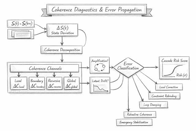
This diagram provides a structural visualisation of the coherence-diagnostic operator implemented by the flow. It should be read top-down and left-to-right, but conceptually it represents a projection through coherence space, not a simple procedural pipeline. Each region of the diagram corresponds to a distinct analytical layer in the diagnostic hierarchy.
The diagram begins with two successive system states, defining a discrete temporal slice. The subtraction operator establishes that change has occurred, but deliberately does not interpret that change as error. This reflects the foundational assumption of the framework: change is not failure.
This layer corresponds to the difference operator in the flow and exists solely to trigger structural analysis.
Coherence Decomposition
Here, raw deviation is projected out of state space and into coherence space. This block represents the diagnostic operator that maps into domain-specific coherence residuals. Visually, it acts as a lens through which deviation is re-expressed in terms of structural alignment.
Importantly, this step discards magnitude as a primary diagnostic and preserves topological relevance.
This block is the core diagnostic domain. Each channel represents a distinct mechanism by which deviation can destabilise the system:
The horizontal grouping indicates that these channels are evaluated in parallel, not sequentially. Dominance of one channel over others determines the governing error-propagation regime.
These detectors represent non-local temporal phenomena that cannot be inferred from a single state difference:
Their placement after coherence decomposition but before classification reflects that they act on coherence trajectories, not raw state.
The diamond denotes a regime resolution operator, not a branching decision tree. At this point, evidence from coherence channels, invariant stress, amplification, and drift is integrated to resolve the dominant propagation regime.
The geometry reflects exclusivity: once a higher-order regime (e.g. recursive or global) is detected, lower-order interpretations are subsumed. This aligns with the flow’s maximal-order classification rule.
This block represents a predictive estimator, not a diagnostic metric. The sigmoid curve emphasises threshold behaviour: small increases in coherence stress can produce disproportionate increases in cascade probability once amplification and invariant violations are present.
Risk is computed as a function of structure, not error size, reflecting the framework’s anticipatory intent.
The fan-out indicates that intervention is conditional on regime, not optional. Each intervention operates at a specific structural layer:
The vertical ordering reflects increasing structural depth. The diagram visually enforces the rule that corrective action must operate at or above the layer where coherence loss originates.
The diagram as a whole should be interpreted as a coherence-space funnel:
Raw change → structural decomposition → propagation detection → regime resolution → topology-matched control
It explicitly rejects the classical “detect error → correct output” paradigm and replaces it with structural diagnosis followed by regime-consistent intervention.
This diagram implements a visual grammar for coherence diagnostics: it shows how deviation is transformed into structural evidence, how hidden amplification and drift are surfaced, how error regimes are resolved by dominance rather than enumeration, and how corrective action is constrained by coherence topology.
It is therefore not an illustration of control flow, but a map of causal responsibility within complex systems
This section establishes a one-to-one correspondence between the visual elements of the diagram and the formal components of the Flow Algebra specification CoherenceDiagnosticsAndErrorPropagation v1.0. The diagram should be understood as a lossy but faithful projection of the flow into visual form: no new logic is introduced, and no formal dependency is omitted.
Top-left paired state blocks labelled and
io.inputs:
  state_t
  state_t1
These blocks represent the temporal diagnostic boundary of the flow. The diagram makes explicit that diagnostics are defined between states, not at a single snapshot. No assumptions are made about optimality, correctness, or intent—only that a transition occurred.
Box labelled “ΔS(t) — State Deviation”
transform: ExtractLocalDeviation
rule: ΔS(t) = state_t1 − state_t
This box corresponds exactly to the discrete difference operator in the flow. The diagram visually isolates this step to emphasise that raw deviation is not yet classified as error. It is merely the triggering signal for coherence analysis.
Intermediate block labelled “Coherence Decomposition”
transform: DecomposeCoherence
output: ΔC(t)
This block corresponds to the projection operator
\[ \Pi\!\left(\Delta S(t)\right) = \Delta C(t) \]
The diagram places this centrally to indicate that all subsequent logic operates in coherence space, not state space.
Grouped boxes:
state:
  ΔC(t):
    components:
      - ΔC_local
      - ΔC_boundary
      - ΔC_recursive
      - ΔC_global
This block is a direct visualisation of the coherence residual vector. The parallel layout reflects that these components are evaluated simultaneously, not hierarchically. The diagram explicitly encodes the flow’s rejection of scalar error metrics in favour of structural decomposition.
Loop icon labelled “Amplification?”
transform: DetectAmplification
output: amplification_flag
The loop symbol is not decorative: it encodes recursive gain under feedback topology. This block visually marks the transition from linear to nonlinear propagation regimes, corresponding exactly to the flow’s amplification detection logic over the history window.
Downward-sloping curve labelled “Latent Drift?”
transform: DetectLatentDrift
output: latent_drift
This element corresponds to the detection of monotonic global coherence decay despite small . Its separation from amplification reflects the flow’s distinction between feedback-driven instability and reference-frame erosion.
Diamond labelled “Error Classification”
classification:
  LocalError
  BoundaryError
  RecursiveError
  GlobalDrift
  PhaseTransition
The diamond symbol denotes a regime resolution operator, not a decision tree. The diagram compresses the flow’s maximal-order classification rule: the resolved class corresponds to the highest structural order of coherence failure detected.
Sigmoid curve labelled “Cascade Risk Score”
monitors:
  CascadeRisk
This element visualises the risk estimator defined in the monitors section. The sigmoid curve encodes threshold behaviour and nonlinearity, reinforcing that cascade probability increases sharply once recursive amplification and invariant stress coexist.
intervention:
  if error_class == ...
Each intervention block maps directly to a regime-consistent control class. The vertical ordering in the diagram mirrors increasing structural depth of intervention, enforcing the flow’s rule that control must act at or above the layer where coherence loss originates.
Structural compression of the full flow.
Executable diagnostic specification.
Every arrow in the diagram corresponds to a dependency defined in the flow. Every block corresponds to either:
No causal path exists in the diagram that is not defined in the Flow Algebra, and no critical flow dependency is omitted from the diagram.
The diagram is a coherence-space projection of CoherenceDiagnosticsAndErrorPropagation v1.0, mapping temporal state deviation into domain-specific coherence residuals, surfacing amplification and latent drift phenomena, resolving the dominant propagation regime, estimating cascade risk as a function of structural stress, and constraining intervention to regime-consistent control classes.
It is therefore a faithful visual encoding of the flow’s diagnostic and control logic, not an illustrative abstraction.
This tri-mapping establishes a three-layer equivalence:
Each row corresponds to a single conceptual operator in the model. No row is decorative; each is required for closure of the diagnostic framework.
| Flow Element | Equation | Interpretation |
|---|---|---|
state_t, state_t1
|
𝑆 ( 𝑡 ) , 𝑆 ( 𝑡 + 1 )
|
Discrete temporal slice
defining the diagnostic window. Establishes change without implying error. |
| Flow Element | Equation | Interpretation |
|---|---|---|
ExtractLocalDeviation<.code>
|
Δ 𝑆 ( 𝑡 ) = 𝑆 ( 𝑡 + 1 ) − 𝑆 ( 𝑡 )
|
Difference operator defining raw
deviation. Serves only as a trigger for structural analysis, not a failure metric. |
| Flow Element | Equation | Interpretation |
|---|---|---|
DecomposeCoherence
|
Π ( Δ 𝑆 ) = Δ 𝐶 ( 𝑡 )
|
Projection from state space
into coherence space. Re-expresses deviation in structurally meaningful domains. |
\[ \Delta C(t) = \begin{bmatrix} \Delta C_{\mathrm{local}}(t) \\ \Delta C_{\mathrm{boundary}}(t) \\ \Delta C_{\mathrm{recursive}}(t) \\ \Delta C_{\mathrm{global}}(t) \end{bmatrix} \]
| Flow Element | Equation | Interpretation |
|---|---|---|
ΔC_local
|
𝑓 local ( Δ 𝑆 )
|
Measures internal consistency |
| Flow Element | Equation | Interpretation |
|---|---|---|
ΔC_boundary
|
𝑓 boundary ( Δ 𝑆 , 𝐼 )
|
Measures stress on
invariants and boundary conditions. Indicates deformation of admissible state manifold. |
| Flow Element | Equation | Interpretation |
|---|---|---|
ΔC_recursive
|
𝑓 recursive ( Δ 𝑆 , 𝐺 )
|
Measures coupling of deviation
into feedback topology. Determines amplification potential. |
| Flow Element | Equation | Interpretation |
|---|---|---|
ΔC_global
|
∥ Δ 𝐶 ( 𝑡 ) ∥ 𝑤
|
Weighted coherence norm
capturing reference-frame stability across the system. |
| Flow Element | Equation | Interpretation |
|---|---|---|
C_i(t)
|
𝐶 𝑖 ( 𝑡 ) ∈ [ 0 , 1 ]
|
Order parameters encoding
alignment within each coherence domain. |
Gradient form:
\[ \nabla C_i(t) = C_i(t+1) - C_i(t) \]
| Flow Element | Equation | Interpretation |
|---|---|---|
invariants
|
𝑆 ( 𝑡 ) ∈ 𝑀 𝑖
|
Hard constraints defining |
| Flow Element | Equation | Interpretation |
|---|---|---|
DetectAmplification
|
⟨ Δ 𝐶 recursive ⟩ 𝑇 > 𝜏 𝑟
|
Detects transition to
feedback-dominated, nonlinear error propagation. |
| Flow Element | Equation | Interpretation |
|---|---|---|
DetectLatentDrift
|
∇ 𝐶 global ( 𝑡 ) < 0 ∧ ∥ Δ 𝑆 ∥ ≪ 𝜖
|
Detects silent degradation
of reference frame prior to visible failure. |
| Flow Element | Equation | Interpretation |
|---|---|---|
classification
|
Regime = max ( 𝑅 𝑖 )
|
Resolves dominant propagation
law based on highest-order coherence failure. |
\[ \mathcal{R} \;\equiv\; \{\mathrm{Local}, \mathrm{Boundary}, \mathrm{Recursive}, \mathrm{Global}\} \]
| Flow Element | Equation | Interpretation |
|---|---|---|
CascadeRisk
|
𝜎 ( Δ 𝐶 global + 𝑔 Δ 𝐶 recursive + 𝑁 inv )
|
Predictive estimate
of cascade probability, based on structural stress and feedback gain. |
| Flow Element | Equation | Interpretation |
|---|---|---|
intervention
|
𝑅 → 𝐴 ≥ 𝑅
|
Restricts corrective
action to control classes operating at or above detected regime order. |
| Flow Element | Equation | Interpretation |
|---|---|---|
termination.safe
|
𝐶 global ≥ 𝜏 recover
|
Certifies return to
a stable coherence basin. |
termination.unstable
|
( C_{\text{global}} < \tau_{\text{global}} \land
|
\mathcal{I}_{\text{violated}}
|
The Flow Algebra specification, its mathematical formalisation, and the diagnostic diagram form a closed triad: the flow defines the operator, the equations define its action, and the diagram encodes causal structure. Together they implement a coherence-theoretic diagnostic framework in which error is treated as a structural signal, propagation is governed by constraint and feedback topology, and correction is restricted to regime-consistent control layers.