Chapter 6
Flow Algebra in Systems Engineering
Flow Algebra
Author: Mark Higgins
Revised Date: 11 February 2026
Author: Mark Higgins
Every engineered system evolves in time — a process of state change guided by control and feedback.
Traditional mathematics describes such systems through differential equations or simulation code.
Flow Algebra, however, abstracts this behaviour in readable, composable form:
state temperature = 25
param target = 30
transition regulate:
    when temperature < target → temperature += gain * (target - temperature)
    when temperature > target → temperature -= gain * (temperature - target)
This single block captures the same logic as a control algorithm, yet remains human-readable and adaptable.
Engineers can directly express what the system should do, not just how it does it.
In automation, Flow Algebra defines processes as declarative flows rather than procedural tasks.
Each process step becomes a state, and each change a transition.
flow "AssemblyLine"

state conveyor = idle
state arm = parked
state part_ready = false

transition process:
    when sensor.detect(part) → part_ready = true
    when part_ready → arm.pick(), conveyor.move()
This abstraction allows engineers to monitor, simulate, and optimise processes without rewriting control code.
Flow blocks can be exported into automation platforms or embedded into microcontroller logic.
Scientific systems often require coupling of multiple evolving variables — temperature, pressure, population, or chemical concentration.
Flow Algebra naturally expresses these interdependencies:
state pressure = 101
state volume = 1.0
param n = 1.0
param R = 8.314
observable temperature = (pressure * volume) / (n * R)
Each update cycle can simulate physical change while preserving mathematical transparency.
The model becomes a readable bridge between human intuition and computational simulation.
Engineering stability depends on feedback.
Flow Algebra encodes this as explicit causal links between observables and actions:
observable error = target - measured
transition control:
    actuator_signal = Kp * error + Ki * ∑error + Kd * Δerror
The flow syntax expresses PID-like control behaviour directly — no need for nested code structures.
Feedback loops thus become first-class citizens within the system model.
Modern engineering increasingly merges physical systems with synthetic intelligence.
Flow Algebra integrates seamlessly with AI or recursion engines by serving as both description and governance layer.
An AI engine can read and modify flow definitions in real time, allowing systems to learn, predict, and stabilise autonomously.
flow "AdaptiveMotor"
state speed = 0
observable drift = target - speed
ai.observe(drift)
ai.learn(rule = adjust_gain(drift))
apply(ai.output)
Here, the recursion engine acts as a cognitive layer — adjusting gain dynamically while preserving defined invariants.
This ensures machine learning remains constrained by engineering logic rather than arbitrary exploration.
Flow Algebra natively supports recursion — systems can describe and refine themselves.
For example, a network control model may generate new flow definitions for its subsystems based on performance metrics:
transition optimise:
    if load > threshold:
        spawn(flow "SubnodeBalancer" with params {capacity = load/2})
Recursive definition and spawning allow scalable, self-structuring architectures — a key principle in modern distributed design.
flow "SmartPump"

state pressure = 80
param target = 100
param gain = 0.1
observable drift = target - pressure

monitor safety:
    when |drift| > 50 → alert("Pressure anomaly")

transition regulate:
    pressure' = pressure + gain * drift
    update(pressure = pressure')

ai.observe(pressure)
ai.learn(rule = adjust_gain(drift))
limit when |drift| < 0.1 → stop
This describes an adaptive hydraulic controller with built-in monitoring, feedback, and AI learning integration — in less than a dozen lines of Flow Algebra.
Flow Algebra offers systems engineers:
By embedding coherence, feedback, and recursion directly into the syntax, Flow Algebra transforms system engineering into a readable, self-correcting discipline — one where every process knows how to describe, test, and evolve itself.
Flow Algebra provides a complete grammar for system design.
In engineering form, it becomes a control logic that unites sensors, actuators, and decision layers under a single rule: every process must preserve coherence through feedback.
The following formalism expresses that rule mathematically.
System Definition
\[ F = (S, P, T, M) \]
\[ \dot{S} = T(S, P) - K\,M(S) \]
where \(K\) is the feedback gain mapping monitored deviation into corrective control action.
Discrete Implementation
\[ S_{t+1} = S_t + T(S_t, P)\,\Delta t - K\,M(S_t)\,\Delta t \]
Error Definition and Correction
\[ E_t = \lVert S_t - S^* \rVert, \qquad S_{t+1} = S_t - G(E_t) \]
where \(S^*\) is the desired equilibrium and \(G\) is a control function determining adjustment rate.
Cascaded Subsystems
For hierarchical or modular engineering:
\[ S = \{ S^{(1)}, S^{(2)}, \dots, S^{(N)} \}, \quad T = \operatorname{blkdiag}\!\big(T^{(1)}, \dots, T^{(N)}\big), \quad M = \operatorname{blkdiag}\!\big(M^{(1)}, \dots, M^{(N)}\big) \]
Each subsystem operates locally while coherence is maintained through a shared invariant:
\[ I(S) = \sum_{i=1}^{N} I^{(i)}(S^{(i)}) = \text{constant} \]
Adaptive Parameter Update (Learning Layer)
\[ P_{t+1} = P_t + L(M(S_t)) \]
where \(L\) is a learning or adaptation function driven by monitor feedback, enabling systems to self-tune.
Stability Requirement
\[ \frac{dE_t}{dt} \le 0, \qquad \lim_{t \to \infty} E_t = 0 \]
ensures controlled processes converge to steady operation.
AI–System Coupling
In adaptive or AI-assisted control:
\[ a_t = f_{\text{AI}}(O_t), \qquad S_{t+1} = T(S_t, a_t, P) \]
AI modifies action \(a_t\) based on observation \(O_t\), but all updates are constrained by coherence monitors:
\[ M(S_t, a_t) = 0 \quad \text{for stable operation.} \]
In Flow Algebra, machines, controllers, and algorithms are not separate layers but parts of a single recursive system.
The same feedback logic that stabilises a circuit also governs an AI’s decision process.
A coherent system is one that measures itself, corrects itself, and evolves without losing structure — the defining principle of engineering through coherence.
Flow Algebra describes automation not as sequences of commands but as structured feedback networks.
Each actuator, sensor, and controller is a node within a coherent flow, communicating through transitions that preserve system balance.
1. Process Loop Definition
For an automated process:
\[ F_p = (S_p, P_p, T_p, M_p) \]
Basic Closed-Loop Form
\[ \dot{S}_p = T_p(S_p, P_p) - K_p\,M_p(S_p) \]
2. Example — Conveyor and Robotic Arm System
Let
\[ S_p = \begin{bmatrix} x_c \\ \theta_a \end{bmatrix}, \qquad P_p = \begin{bmatrix} v_{\text{target}} \\ \theta_{\text{target}} \end{bmatrix} \]
where \(x_c\) is the conveyor position and \(\theta_a\) the robotic arm angle.
Transition (Process Operator)
\[ T_p(S_p, P_p) = \begin{bmatrix} v_{\text{target}} - k_v (x_c - x^*) \\ \omega_{\text{target}} - k_{\theta} (\theta_a - \theta^*) \end{bmatrix} \]
Monitor Functions
\[ M_p(S_p) = \begin{bmatrix} x_c - x^* \\ \theta_a - \theta^* \end{bmatrix} \]
Control Law
\[ \dot{S}_p = T_p(S_p, P_p) - K_p\,M_p(S_p) \]
where
\[ K_p = \operatorname{diag}(k_v, k_\theta) \]
acts as proportional correction for each axis.
3. Coordinated Sub-Flows
Each actuator is a sub-flow \(F_i\).
The complete process is:
\[ F_{\text{system}} = \{ F_1, F_2, \dots, F_N \}, \qquad M_{\text{system}} = \sum_{i} w_i\,M_i(S_i) \]
where \(w_i\) are weighting coefficients for local monitor influence.
Coherence across all sub-flows is preserved when:
\[ \lVert M_{\text{system}} \rVert \le \varepsilon \;\Rightarrow\; \text{Process Stable.} \]
4. Automation Hierarchy
Process automation forms a three-level recursive flow:
\[ P_{t+1} = P_t + L(M_{\text{system}}) \]
where \(L\) defines adaptation rules or learning from operational drift.
5. Fault Detection and Recovery
A system fault occurs when monitor deviation exceeds tolerance:
\[ \lVert M_i(S_i) \rVert > \varepsilon_i \;\Rightarrow\; \text{trigger recovery flow } T_{r,i} \]
Each recovery flow is a temporary reconfiguration:
\[ S_i \rightarrow S_i' = R_i(S_i) \quad \text{such that} \quad M_i(S_i') = 0 \]
If recovery fails after attempts:
\[ M_i(S_i') > \varepsilon_i \;\Rightarrow\; \text{halt process and escalate to supervisory flow.} \]
Reflection on Automated Coherence
In Flow Algebra, automation is not programmed — it is expressed.
The same grammar that defines a physical system defines its response, its feedback, and its ethics of operation.
Every actuator is a transition, every sensor a monitor, every control loop a flow seeking coherence.
Thus, the act of automation itself becomes a dynamic equation of balance:
\[ \lim_{t \to \infty} M_{\text{system}}(S_t) = 0 \]
— a factory, a machine, or a network finding stability through recursive self-awareness.
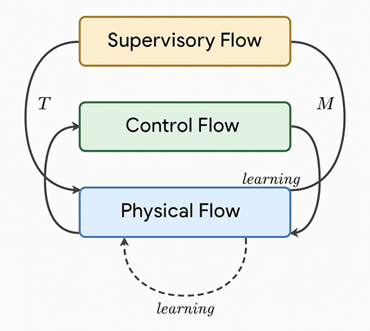
Each component — sensors, actuators, controller, and supervisory AI — is represented as a distinct flow block communicating through monitored coherence.
1. Physical Layer
2. Control Layer
3. Supervisory Layer
4. Coherence Loop
\[ \lVert M_{\text{system}}(S_t) \rVert \le \varepsilon \]
| Symbol | Meaning | Typical Domain |
|---|---|---|
|
\(S_p\) |
Process state vector \([x_c, \theta_a]^{\top}\) |
Physical space |
|
\(P_p\) |
Control parameters (targets) |
Supervisor layer |
|
\(T_p\) |
Transition / actuator function |
Control logic |
|
\(M_p\) |
Local monitor measuring deviation |
Sensor feedback |
|
\(K_p\) |
Gain matrix \(\operatorname{diag}(k_v, k_\theta)\) |
Control tuning
|
|
\(x_c, \; x^*\) |
Conveyor position / target
|
\(m\) \text{ (scalar)} |
|
\(\theta_a, \; \theta^*\) |
Arm angle / target
|
rad
|
|
\(L(M_{\text{system}})\) |
Learning update rule
|
Supervisory
|
|
\(f_{\text{AI}}(O_t)\) |
AI observer generating corrective intent
|
Cognitive module
|
|
\(I(S)\) |
Global invariant (energy/timing constraint)
|
System-wide
|
Summary Equation
\[ \dot{S}_{\text{system}} = T_{\text{physical}}(S, P) - K_{\text{control}}\,M_{\text{sensors}}(S) - K_{\text{AI}}\,M_{\text{system}}(S, P) \]
which unites mechanical, electronic, and intelligent processes under one coherent grammar.